Conditional Probability

The probability of an event once we know that another event has occurred.

Prerequisites: Introduction to Probability.

The conditional probability of an event $A$ given an event $B$, written $P(A \mid B)$, is the probability that $A$ happens when we already know that $B$ has happened. It is how probabilities are updated in the light of new information, and almost every realistic probability question involves it: the chance of rain given a cloudy morning, the chance of a disease given a positive test, the chance of default given a borrower’s income.

Intuition

Knowing that $B$ happened rules out every outcome outside $B$. What remains is a smaller world, and within that world we ask how much of it belongs to $A$.

Draw one card from a well-shuffled standard deck of 52 cards. The probability that it is a king is $4/52 = 1/13$. Now suppose a friend peeks and tells you the card is a face card (a jack, queen, or king). There are only 12 face cards, and 4 of them are kings, so the probability of a king given this information is $4/12 = 1/3$. The information shrank the set of possibilities from 52 cards to 12, and kings make up a larger share of the smaller set.

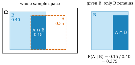
The picture below shows the same idea with areas. Think of the sample space $\Omega$ as a rectangle of total area 1, and of each event as a region whose area is its probability. Conditioning on $B$ throws away everything outside $B$; the conditional probability of $A$ is the fraction of $B$’s area that is also inside $A$.

Definition

Let $A$ and $B$ be events with $P(B) > 0$. The conditional probability of $A$ given $B$ is

$$P(A \mid B) = \frac{P(A \cap B)}{P(B)}.$$

Here $A \cap B$ is the event “both $A$ and $B$ happen”. In words: of all the probability sitting on $B$, what fraction also lies in $A$?

Some remarks:

• The condition $P(B) > 0$ is needed because we divide by $P(B)$. Conditioning on an event of probability zero needs a more careful treatment that is beyond this article.
• For a fixed $B$, the function $A \mapsto P(A \mid B)$ obeys all the axioms of probability. In particular, $P(A^c \mid B) = 1 - P(A \mid B)$, and $P(B \mid B) = 1$. Conditioning simply produces a new probability on a smaller world.
• When all outcomes are equally likely, the definition reduces to counting inside $B$: $P(A \mid B) = |A \cap B| / |B|$, as in the card example.

The multiplication rule

Rearranging the definition gives a rule for the probability that two events both happen:

$$P(A \cap B) = P(B)\, P(A \mid B) = P(A)\, P(B \mid A).$$

This is often the natural way to compute a joint probability step by step. For example, draw two cards without replacement. The probability that both are aces is

$$P(\text{1st ace}) \cdot P(\text{2nd ace} \mid \text{1st ace}) = \frac{4}{52} \cdot \frac{3}{51} = \frac{1}{221} \approx 0.0045.$$

The second factor is a conditional probability: once an ace has been removed, 3 aces remain among 51 cards.

The law of total probability

Sometimes $P(A)$ is hard to find directly but easy to find in each of several separate cases. Suppose the events $B_1, B_2, \dots, B_k$ form a partition of $\Omega$: they are mutually exclusive and together cover every outcome, so exactly one of them happens. Then

$$P(A) = \sum_{i=1}^k P(A \mid B_i)\, P(B_i).$$

The simplest partition is $B$ and its complement $B^c$:

$$P(A) = P(A \mid B)\, P(B) + P(A \mid B^c)\, P(B^c).$$

This says that the overall probability of $A$ is a weighted average of its conditional probabilities in each case, weighted by how likely each case is. It follows from splitting $A$ into the disjoint pieces $A \cap B_i$, adding their probabilities, and applying the multiplication rule to each piece.

Worked example

A survey of 200 households records whether each owns a dog and whether it owns a cat.

Choose one of these households at random. Let $C$ be “owns a cat” and $D$ be “owns a dog”.

Step 1: unconditional probabilities. From the totals, $P(C) = 70/200 = 0.35$ and $P(D) = 80/200 = 0.40$. Both owning a dog and a cat: $P(C \cap D) = 30/200 = 0.15$. (These are the numbers in the figure above, with $A = C$ and $B = D$.)

Step 2: condition on owning a dog. Restrict attention to the 80 dog-owning households. Of these, 30 own a cat:

$$P(C \mid D) = \frac{P(C \cap D)}{P(D)} = \frac{0.15}{0.40} = 0.375.$$

Counting directly in the “Dog” row gives the same answer, $30/80 = 0.375$.

Step 3: condition the other way. Among the 70 cat-owning households, 30 own a dog:

$$P(D \mid C) = \frac{30}{70} \approx 0.429.$$

So $P(C \mid D) \ne P(D \mid C)$. The numerator is the same, $30$ households, but the denominators differ: 80 dog owners versus 70 cat owners.

Step 4: check with the law of total probability. Among households without a dog, $P(C \mid D^c) = 40/120 = 1/3$. Then

$$P(C) = P(C \mid D)\,P(D) + P(C \mid D^c)\,P(D^c) = 0.375 \times 0.40 + \tfrac{1}{3} \times 0.60 = 0.15 + 0.20 = 0.35,$$

which matches Step 1.

Common misunderstandings

“P(A | B) is the same as P(B | A).” It is not, and confusing the two (sometimes called the confusion of the inverse) causes serious errors. The probability that a person who has a disease tests positive can be high while the probability that a person who tests positive has the disease is low. Bayes’ theorem is the rule that converts one into the other.

“P(A | B) is the same as P(A ∩ B).” The joint probability $P(A \cap B)$ is measured relative to the whole sample space; the conditional probability is measured relative to $B$ only. In the example, $P(C \cap D) = 0.15$ but $P(C \mid D) = 0.375$.

“Conditioning on B always changes the probability of A.” Not necessarily. If $P(A \mid B) = P(A)$, learning that $B$ happened tells us nothing about $A$. Such events are called independent.

“The vertical bar means division.” $P(A \mid B)$ is read “the probability of $A$ given $B$”. The notation $A \mid B$ on its own is not an event, and $P(A \mid B)$ is not $P(A) / P(B)$.

Further reading

• Joseph K. Blitzstein and Jessica Hwang, Introduction to Probability, 2nd ed., CRC Press, 2019. Covers conditional probability in depth, with many worked examples and common pitfalls.
• David M. Diez, Mine Çetinkaya-Rundel, and Christopher D. Barr, OpenIntro Statistics, 4th ed., 2019. Free online; introduces conditional probability through contingency tables.

Related articles

• Statistical Independence — Two events are independent when knowing that one happened does not change the probability of the other.
• Bayes' Theorem — A rule for reversing a conditional probability, turning P(evidence | hypothesis) into P(hypothesis | evidence).
• Random Variables — A random variable assigns a number to each outcome of a random experiment; its distribution is described by a PMF, a PDF, or a CDF.