Expected Value

The probability-weighted average of a random variable's values, interpreted as its long-run average and as the balance point of its distribution.

Prerequisites: Random Variables.

The expected value (or mean, or expectation) of a random variable is the average of its possible values, each weighted by how probable it is. It is the value you would get, on average, if you could repeat the random experiment many times. The expected value is the most common single-number summary of a distribution, and it is the population counterpart of the familiar sample mean.

Intuition

Roll a fair die many times and average the results. Each face from 1 to 6 comes up about one-sixth of the time, so the average settles down near

1 \cdot \tfrac16 + 2 \cdot \tfrac16 + 3 \cdot \tfrac16 + 4 \cdot \tfrac16 + 5 \cdot \tfrac16 + 6 \cdot \tfrac16 = \tfrac{21}{6} = 3.5.

That number is the expected value of a die roll. It is a weighted average: every value counts in proportion to its probability. The law of large numbers makes the “settles down” claim precise.

Notice that 3.5 is not a possible result of a roll. The expected value is a long-run average, not a prediction of any single outcome.

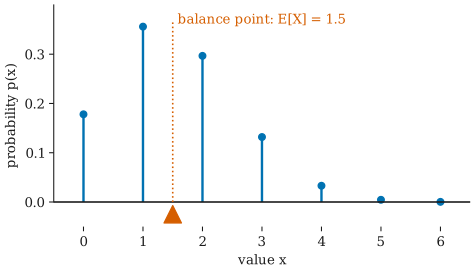
A second, physical picture is just as useful. Imagine the possible values marked on a weightless rod, with a weight at each value proportional to its probability. The expected value is the point where the rod would balance.

Stems for the values 0 to 6 with heights 0.18, 0.36, 0.30, 0.13, 0.03 and two tiny ones; the distribution has a long right tail. A triangle under the axis at 1.5 marks the balance point, which lies between the possible values 1 and 2. — PMF of the number of correct answers when guessing on 6 multiple-choice questions with 4 options each (a binomial distribution with n = 6, p = 0.25). The mean, 1.5, is the balance point; the long right tail pulls it to the right of the most likely value, 1.

Definition

Let $X$ be a random variable. Its expected value is written $\E[X]$ , and often $\mu$ when there is no ambiguity.

Discrete case. If $X$ has probability mass function $p(x) = P(X = x)$ , then

\E[X] = \sum_x x\, p(x),

where the sum runs over all values $X$ can take. Each value is multiplied by its probability, and the results are added.

Continuous case. If $X$ has probability density function $f(x)$ , the sum becomes an integral:

\E[X] = \int_{-\infty}^{\infty} x\, f(x)\, dx.

The density $f(x)$ plays the role of the probabilities, and the integral is a continuous weighted average.

When it exists. The expected value is defined only when the sum or integral converges absolutely, that is, when $\sum_x |x|\,p(x)$ or $\int |x| f(x)\,dx$ is finite. For every distribution with finitely many values this is automatic. Some heavy-tailed distributions, such as the Cauchy distribution, have no expected value at all: the averages of repeated samples never settle down.

Expected value of a function

Often we need the expected value of a quantity computed from $X$ , such as $X^2$ or a payoff that depends on $X$ . For a function $g$ ,

\E[g(X)] = \sum_x g(x)\, p(x) \qquad \text{or} \qquad \E[g(X)] = \int_{-\infty}^{\infty} g(x)\, f(x)\, dx.

We apply $g$ to each value but keep the original probabilities. There is no need to work out the distribution of $g(X)$ first.

Worked example

A game. You pay 1 dollar to roll a fair die. If it shows a 6 you receive 5 dollars; otherwise you receive nothing. Let $W$ be your net winnings in dollars. Then $W = 4$ with probability $1/6$ and $W = -1$ with probability $5/6$ , so

\E[W] = 4 \cdot \tfrac{1}{6} + (-1) \cdot \tfrac{5}{6} = -\tfrac{1}{6} \approx -0.17.

On average you lose about 17 cents per game. Over 600 games you should expect to be down about 100 dollars, although any particular sequence of games will differ.

The distribution in the figure. Guessing at random on 6 questions, each with 4 options, the number $X$ of correct answers has these probabilities:

$x$	0	1	2	3	4	5	6
$p(x) \times 4096$	729	1458	1215	540	135	18	1

(These come from the binomial distribution with $n = 6$ trials and success probability $p = 0.25$ .) Then

\E[X] = \frac{0 \cdot 729 + 1 \cdot 1458 + 2 \cdot 1215 + 3 \cdot 540 + 4 \cdot 135 + 5 \cdot 18 + 6 \cdot 1}{4096} = \frac{6144}{4096} = 1.5.

The most likely value is 1, but the small probabilities on 3, 4, 5, and 6 sit far to the right and pull the balance point to 1.5.

A continuous example. If $X$ is uniformly distributed on $[0, 1]$ , its density is $f(x) = 1$ there, and

\E[X] = \int_0^1 x \cdot 1 \, dx = \left[\tfrac{x^2}{2}\right]_0^1 = \tfrac12,

the midpoint, as symmetry suggests.

Linearity of expectation

The single most useful property of expected value is that it is linear. For any random variables $X$ and $Y$ and constants $a$ and $b$ ,

\E[aX + b] = a\,\E[X] + b, \qquad \E[X + Y] = \E[X] + \E[Y].

The first rule says that rescaling and shifting a random variable rescales and shifts its mean in the same way. Converting temperatures from Celsius to Fahrenheit, $F = 1.8C + 32$ , converts the expected temperature by the same formula.

The second rule says that the expected value of a sum is the sum of the expected values. Crucially, this holds whether or not $X$ and $Y$ are independent. More generally, $\E[X_1 + \cdots + X_n] = \E[X_1] + \cdots + \E[X_n]$ .

For discrete variables the first rule follows directly from the definition:

\E[aX + b] = \sum_x (ax + b)\,p(x) = a \sum_x x\,p(x) + b \sum_x p(x) = a\,\E[X] + b,

using $\sum_x p(x) = 1$ .

Example: two dice. The sum $S$ of two dice has the triangular distribution shown in the random variables article. Instead of using that distribution, write $S = X_1 + X_2$ , where $X_1$ and $X_2$ are the two dice. Then $\E[S] = 3.5 + 3.5 = 7$ .

Example: counting with indicators. How many sixes do you expect in 10 rolls of a die? Let $I_j$ be $1$ if roll $j$ is a six and $0$ otherwise. Each $I_j$ has $\E[I_j] = 1 \cdot \tfrac16 + 0 \cdot \tfrac56 = \tfrac16$ . The number of sixes is $I_1 + \cdots + I_{10}$ , so its expected value is $10 \times \tfrac16 = \tfrac{10}{6} \approx 1.67$ . This trick of writing a count as a sum of 0–1 indicators makes many hard-looking expectations easy, even when the indicators are dependent.

Linearity is also the reason that the sample mean $\bar{X}$ of a random sample has the same expected value as each observation, a fact used throughout point estimation.

Common misunderstandings

“The expected value is the most likely value.” Not in general. For the guessing example, the most likely value is 1 but the mean is 1.5. For a single die every value is equally likely, and the mean, 3.5, is not even a possible value.

“The expected value is what will happen.” It is a long-run average. In a single play of the game above you either win 4 dollars or lose 1 dollar; you never lose exactly 17 cents.

“E[g(X)] = g(E[X]).” This is false unless $g$ is linear. For a die, $\E[X^2] = (1 + 4 + 9 + 16 + 25 + 36)/6 = 91/6 \approx 15.17$ , while $(\E[X])^2 = 3.5^2 = 12.25$ . The gap between these two numbers is exactly the variance of a die roll.

“E[XY] = E[X] E[Y].” This product rule needs extra assumptions; it holds when $X$ and $Y$ are independent, but not in general. The difference $\E[XY] - \E[X]\E[Y]$ is the covariance. Linearity for sums needs no such assumption.

“The mean is the middle value.” The middle value is the median. For skewed distributions the mean is pulled toward the long tail, as the figure shows.