Point Estimation

Using a single number computed from a sample to estimate an unknown population parameter, and judging how good that rule is.

Prerequisites: Sampling Distributions, Expected Value, Variance of a Random Variable.

Point estimation is the use of sample data to produce a single best guess, a point estimate, for an unknown quantity describing a population, such as its mean, a proportion, or a variance. The sample mean as a guess for the population mean is the most familiar example.

Since any guess from a random sample will be somewhat off, the important question is not whether one estimate is right, but whether the rule that produced it tends to land close to the truth. The ideas of bias, variance, and mean squared error make that question precise, and they let us compare different ways of estimating the same thing.

Parameters, estimators, and estimates

A parameter, written generically as $\theta$ (theta), is a fixed but unknown number describing the population: the mean $\mu$, the variance $\sigma^2$, the proportion $p$ of voters supporting a candidate.

An estimator $\hat{\theta}$ (“theta hat”) is a rule for computing a guess of $\theta$ from the data $X_1, \dots, X_n$. Because the data are random, an estimator is a random variable with a sampling distribution.

An estimate is the number you get when you apply the rule to the data you actually observed.

For example, the sample mean $\bar{X} = \frac{1}{n}\sum_{i=1}^n X_i$ is an estimator of $\mu$. If five measured waiting times average 2.3 minutes, then 2.3 is an estimate. Asking “is 2.3 biased?” makes no sense; asking “is $\bar{X}$ biased?” does, because it is a question about how the rule behaves over all the samples that could have occurred.

Bias, variance, and mean squared error

Picture the sampling distribution of an estimator. Two things determine whether it is a good one: where its distribution is centred, and how spread out it is.

Bias measures the centre. It is the difference between the estimator’s average value and the true parameter:

$$\operatorname{Bias}(\hat{\theta}) = \E[\hat{\theta}] - \theta.$$

An estimator with zero bias for every possible value of $\theta$ is called unbiased: on average, over many samples, it hits the target.

Variance measures the spread: $\Var(\hat{\theta})$ says how much the estimate changes from sample to sample. Its square root is the standard error of the estimator.

Mean squared error (MSE) combines the two into a single measure of how far the estimate typically lands from the truth:

$$\operatorname{MSE}(\hat{\theta}) = \E\big[(\hat{\theta} - \theta)^2\big].$$

The bias–variance decomposition

The MSE splits exactly into a variance part and a bias part:

$$\operatorname{MSE}(\hat{\theta}) = \Var(\hat{\theta}) + \operatorname{Bias}(\hat{\theta})^2.$$

To see why, write $m = \E[\hat{\theta}]$ and add and subtract it inside the square:

$$(\hat{\theta} - \theta)^2 = (\hat{\theta} - m)^2 + 2(\hat{\theta} - m)(m - \theta) + (m - \theta)^2.$$

Now take expectations term by term. The first term gives $\E[(\hat{\theta} - m)^2] = \Var(\hat{\theta})$. In the middle term, $m - \theta$ is a constant and $\E[\hat{\theta} - m] = 0$, so it vanishes. The last term is the constant $(m - \theta)^2 = \operatorname{Bias}(\hat{\theta})^2$.

The decomposition says there are two ways to be wrong: systematically (bias) and randomly (variance). Reducing one often increases the other.

The bias–variance tradeoff

An unbiased estimator is not automatically the best one. Accepting a small bias can sometimes buy a large reduction in variance, and so a smaller MSE.

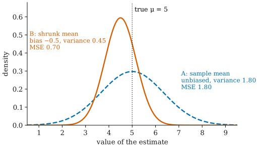
In the figure, the population mean is $\mu = 5$, and each sample has $n = 5$ observations from a normal population with $\sigma = 3$. Estimator A is the sample mean. Estimator B, $(\bar{X} + 4)/2$, averages the sample mean with a prior guess of 4. Then:

• A is unbiased, with variance $\sigma^2/n = 9/5 = 1.8$, so its MSE is $1.8$.
• B has mean $(5 + 4)/2 = 4.5$, so its bias is $-0.5$. Its variance is $\tfrac{1}{4} \cdot 1.8 = 0.45$. Its MSE is $0.45 + 0.5^2 = 0.70$.

Here the biased estimator is better on average. But it is better only because the guess of 4 happened to be close to the truth; if the true mean were 10, B’s bias would be $-3$ and its MSE about 9.45, far worse than A. Shrinking towards a guess helps when the guess is good and the sample is small. This tradeoff appears throughout statistics and machine learning, for example in regularized regression.

Consistency

An estimator is consistent if it gets arbitrarily close to $\theta$ as the sample size grows: for every $\varepsilon > 0$,

$$P\big(|\hat{\theta}_n - \theta| > \varepsilon\big) \to 0 \quad \text{as } n \to \infty,$$

where $\hat{\theta}_n$ is the estimator computed from $n$ observations. A convenient sufficient condition is that both the bias and the variance go to zero as $n$ grows, because then the MSE goes to zero.

The sample mean is consistent for $\mu$: this is the law of large numbers. Consistency is a minimal requirement. An estimator that does not home in on the truth even with unlimited data is rarely worth using. Bias and consistency are different properties: an estimator can be biased for every finite $n$ and still consistent, as the next example shows.

Example: estimating a variance

Let $X_1, \dots, X_n$ be iid with mean $\mu$ and variance $\sigma^2$. A natural estimator of $\sigma^2$ averages the squared deviations from the sample mean:

$$\hat{\sigma}^2 = \frac{1}{n} \sum_{i=1}^n (X_i - \bar{X})^2.$$

Its expected value. Expanding the square shows that $\sum_{i}(X_i - \bar{X})^2 = \sum_i X_i^2 - n\bar{X}^2$. Since $\E[X_i^2] = \sigma^2 + \mu^2$ and $\E[\bar{X}^2] = \Var(\bar{X}) + \mu^2 = \sigma^2/n + \mu^2$,

$$\E\Big[\sum_{i=1}^n (X_i - \bar{X})^2\Big] = n(\sigma^2 + \mu^2) - n\Big(\frac{\sigma^2}{n} + \mu^2\Big) = (n-1)\sigma^2.$$

So $\E[\hat{\sigma}^2] = \frac{n-1}{n}\sigma^2$: the estimator is biased downwards, by $-\sigma^2/n$. The deviations are measured from $\bar{X}$, which is fitted to the same data and so sits closer to them than $\mu$ does. Dividing by $n - 1$ instead gives the unbiased sample variance $s^2$; see variance and standard deviation. Since the bias $-\sigma^2/n$ shrinks to zero, $\hat{\sigma}^2$ is still consistent.

Worked example. Take $n = 5$ observations from a normal population with $\sigma^2 = 1$. For normal data, the variance of $s^2$ is $2\sigma^4/(n-1)$.

1. Unbiased $s^2$: bias $0$, variance $2/4 = 0.5$, so MSE $= 0.5$.
2. Divide-by-$n$ estimator $\hat{\sigma}^2 = \frac{n-1}{n}s^2 = 0.8\,s^2$: bias $0.8 - 1 = -0.2$, variance $0.8^2 \times 0.5 = 0.32$, so MSE $= 0.32 + 0.04 = 0.36$.

The biased estimator has the smaller MSE. Even so, $s^2$ is the standard choice, because unbiasedness is convenient when estimates are combined and because inference methods such as the $t$ test are built around it. Neither is “the correct” estimator; they are optimal by different criteria.

How estimators are constructed

Bias, variance, and MSE judge an estimator once you have one. Two general recipes produce them:

• Method of moments: set sample averages equal to their population counterparts and solve. For example, set $\bar{x}$ equal to $\E[X]$, written in terms of the parameters.
• Maximum likelihood: choose the parameter value under which the observed data are most probable. This is the most widely used general method, and it has good large-sample properties; see maximum likelihood estimation.

A point estimate on its own says nothing about its own uncertainty. Reporting it with a standard error, or as a confidence interval, tells the reader how far off it could plausibly be.

Common misunderstandings

“An unbiased estimator gives the right answer.” It gives the right answer on average over many samples. Any single estimate can be far off, especially if the variance is large.

“Unbiased is always better than biased.” Not if the goal is to be close to the truth. As both examples above show, a slightly biased estimator can have a smaller mean squared error.

“If $s^2$ is unbiased for $\sigma^2$, then $s$ is unbiased for $\sigma$.” It is not: taking a square root does not commute with averaging. For $n = 5$ normal observations, $\E[s] \approx 0.94\,\sigma$. The bias shrinks as $n$ grows, and is usually ignored.

“Bias means the data were collected badly.” Statistical bias is a property of an estimator under an assumed model. Sampling bias, where the sample is not representative of the population, is a different and often more serious problem that no choice of estimator can fix.

Further reading

• Larry Wasserman, All of Statistics: A Concise Course in Statistical Inference, Springer, 2004. A concise treatment of bias, standard error, MSE and consistency.
• George Casella and Roger L. Berger, Statistical Inference, 2nd ed., Duxbury, 2002. The standard graduate-level reference on point estimation, including the method of moments and maximum likelihood.

Related articles

• Likelihood and Maximum Likelihood Estimation — The likelihood measures how well each parameter value explains the observed data; the maximum likelihood estimate is the value that explains them best.
• Confidence Intervals — A range of plausible values for a parameter, produced by a procedure that captures the true value in a stated fraction of repeated samples.
• Variance and Standard Deviation — Measures of how far data values typically lie from their mean, including why the sample variance divides by n − 1.
• Law of Large Numbers — As a sample grows, its average gets closer and closer to the expected value.