Central Limit Theorem

The mean of many independent observations is approximately normally distributed, whatever the shape of the population.

Prerequisites: Sampling Distributions, Normal Distribution, Law of Large Numbers.

The central limit theorem (CLT) says that if you add up or average many independent random quantities with the same distribution, the result is approximately normally distributed, even when the individual quantities are far from normal. The larger the number of quantities, the better the approximation.

This is why the normal distribution is everywhere in statistics. We rarely know the shape of a population, but we often need the distribution of a sample mean in order to build a confidence interval or carry out a hypothesis test. The central limit theorem tells us that, for a large enough sample, that distribution is close to a normal one with a known centre and spread.

Intuition

Roll one fair die and every face from 1 to 6 is equally likely: a flat distribution. Roll two dice and add them, and a total of 7 is six times as likely as a total of 2, because many combinations produce middling totals and only one produces each extreme. With more dice, this effect grows: extreme totals need every die to be extreme together, which is rare, while middling totals can arise in an enormous number of ways. The distribution piles up in the middle and takes on a bell shape.

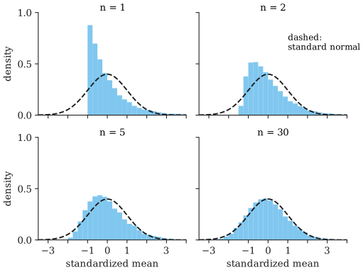
The same happens for skewed variables. The figure below starts with the exponential distribution, which is strongly skewed: it has a peak at zero and a long right tail. Averages of 2 or 5 exponential values are still visibly skewed, but by 30 the histogram is close to the normal curve.

Four histograms of standardized sample means from an exponential population, for sample sizes 1, 2, 5 and 30, each with the standard normal curve drawn dashed. For n equal to 1 the histogram is sharply skewed with a wall at minus 1; it becomes more symmetric as n grows, and at n equal to 30 it nearly matches the normal curve. — Standardized means √n(X̄ − 1) of n independent Exponential(1) values (mean 1, standard deviation 1), for n = 1, 2, 5 and 30, from 20,000 simulated samples each. The dashed curve is the standard normal density. The skewness fades as n grows.

Statement

Let $X_1, X_2, \dots, X_n$ be independent and identically distributed (iid) random variables with mean $\mu$ and finite, positive variance $\sigma^2$ . Let $\bar{X}_n$ be their sample mean.

From the article on sampling distributions, $\bar{X}_n$ has mean $\mu$ and standard error $\sigma/\sqrt{n}$ . Subtracting the mean and dividing by the standard error gives a standardized mean $Z_n$ , which always has mean $0$ and variance $1$ :

Z_n = \frac{\bar{X}_n - \mu}{\sigma / \sqrt{n}} = \frac{\sqrt{n}\,(\bar{X}_n - \mu)}{\sigma}.

Central limit theorem. As $n \to \infty$ , the distribution of $Z_n$ approaches the standard normal distribution: for every real number $z$ ,

P(Z_n \le z) \to \Phi(z),

where $\Phi$ is the cumulative distribution function of the standard normal distribution $\mathcal{N}(0, 1)$ . This is called convergence in distribution.

What this means in practice

For large $n$ we use the approximation

\bar{X}_n \approx \mathcal{N}\!\left(\mu, \frac{\sigma^2}{n}\right),

read as “the sample mean is approximately normal with mean $\mu$ and variance $\sigma^2/n$ ”. Equivalently, the sum $S_n = X_1 + \dots + X_n$ is approximately $\mathcal{N}(n\mu, n\sigma^2)$ .

The centre and spread are not part of the theorem: $\E[\bar{X}_n] = \mu$ and $\Var(\bar{X}_n) = \sigma^2/n$ hold exactly for every $n$ . What the CLT adds is the shape. Without it, we would know how wide the sampling distribution is but not how much probability lies in its tails.

Relation to the law of large numbers

The law of large numbers says $\bar{X}_n$ gets close to $\mu$ . The central limit theorem zooms in on the remaining error $\bar{X}_n - \mu$ : it is typically of size $\sigma/\sqrt{n}$ , and its distribution is approximately normal. Both results describe the same averages at different levels of detail.

Worked example

Waiting times at a service counter are exponentially distributed with mean $\mu = 2$ minutes. For an exponential distribution the standard deviation equals the mean, so $\sigma = 2$ minutes. What is the probability that the average wait of 36 customers exceeds 2.5 minutes?

Step 1: centre and spread of the mean. $\E[\bar{X}] = 2$ and

\operatorname{SE} = \frac{\sigma}{\sqrt{n}} = \frac{2}{\sqrt{36}} = \frac{1}{3} \approx 0.333 \text{ minutes}.

Step 2: standardize. The z-score of 2.5 is

z = \frac{2.5 - 2}{1/3} = 1.5.

Step 3: apply the normal approximation.

P(\bar{X} > 2.5) \approx 1 - \Phi(1.5) \approx 1 - 0.9332 = 0.0668.

So about a 6.7% chance.

Step 4: check against simulation. Simulating 100,000 groups of 36 exponential waiting times gives a proportion of about 0.075 with an average above 2.5 minutes. (Here the exact answer is also available, because a sum of exponential variables has a gamma distribution; it is about 0.074.) The approximation is in the right range but noticeably too small. The reason is the leftover skewness visible in the figure: with an exponential population, even a mean of 36 values has a slightly longer right tail than a normal distribution. In the left tail the error goes the other way: the normal approximation gives $P(\bar{X} < 1.5) \approx 0.067$ , while the exact value is about 0.056.

Why it underlies confidence intervals and tests

Many standard methods have the same structure: compute an estimate, compute its standard error, and use the normal distribution to say how far the estimate is likely to be from the truth. The central limit theorem is what justifies the third step when the data themselves are not normal.

For example, because $\bar{X}_n$ is approximately normal, it lies within $1.96$ standard errors of $\mu$ in about 95% of samples. Turning that statement around gives the familiar interval $\bar{x} \pm 1.96\, s/\sqrt{n}$ for $\mu$ ; see confidence intervals. Similarly, a hypothesis test for a mean compares the observed z-score with the standard normal distribution.

The CLT also explains the normal approximation to the binomial distribution: a binomial count is a sum of independent 0/1 Bernoulli variables, so for many trials it is approximately normal.

Common misunderstandings

“With a large sample, the data become normal.” No. The data have whatever distribution the population has; a large sample of exponential waiting times is still skewed, and its histogram just looks more and more like the exponential density. The CLT is about the sampling distribution of the mean (or sum), the distribution of $\bar{X}$ across repeated samples.

“n ≥ 30 is enough.” This is a rough rule of thumb, not part of the theorem. How large $n$ must be depends on the population. For a symmetric population with light tails, a sample of 10 may already be plenty. For a strongly skewed population, or one with occasional extreme values, 30 may be far too few, and the worked example above shows a visible error even at 36 for a moderately skewed one. Tail probabilities, which are what tests and intervals rely on, are usually the slowest part to become accurate.

“It works for any distribution.” It needs a finite variance. For very heavy-tailed distributions, such as the Cauchy distribution, the sample mean does not become normal however large $n$ is. In practice, data with rare but enormous values (insurance claims, file sizes, wealth) can make the CLT approximation poor for any realistic sample size.

“It works for any sample.” The basic theorem assumes independent observations from one distribution. Versions exist for some dependent or non-identical data, but strongly dependent observations, such as a time series with long memory, can behave very differently.