Sampling Distributions

The distribution of a statistic, such as the sample mean, over all the samples that could have been drawn.

Prerequisites: Populations and Samples, Random Variables, Expected Value, Variance of a Random Variable.

The sampling distribution of a statistic is the distribution of values that statistic would take if we drew sample after sample from the same population and recomputed it each time. A sample mean, a sample proportion, or a sample median is not a fixed number: a different random sample would have given a different value. The sampling distribution describes that variation.

It is the central idea of statistical inference. We almost always see just one sample, but to judge how far our one estimate is likely to be from the truth, we need to know how much the estimate would vary across samples. The standard deviation of the sampling distribution, called the standard error, answers exactly that question.

Intuition

Suppose you want to know the average time customers wait at a café. You cannot time every customer, so you time 25 of them and compute their average. A colleague who times a different 25 customers will get a somewhat different average. A third person gets a third value, and so on.

Two things are true about this collection of averages:

• They scatter around the true population average. Some samples happen to contain more long waits, some fewer, but there is no systematic tendency to land too high or too low.
• They scatter much less than individual waiting times do. A single customer might wait 6 minutes, but for a sample of 25 to average 6 minutes, many customers in the sample would have to wait a long time at once, which is unlikely. Averaging cancels out much of the individual variation.

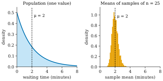
The figure shows this with a simulation. The population on the left is strongly skewed: most waits are short, a few are long. The histogram on the right shows 5,000 sample means, each computed from a fresh sample of 25 waits. They are centred on the population mean, and they are far more tightly concentrated than the individual values. Notice also that the histogram is much more symmetric than the population; that is the central limit theorem at work.

A statistic is a random variable

Here is the key shift in viewpoint. Before the sample is drawn, the observations are unknown, so we model them as random variables $X_1, X_2, \dots, X_n$. A statistic is any quantity computed from the sample. Because it is a function of random variables, a statistic is itself a random variable, and it has its own distribution: its sampling distribution.

Notation distinguishes the two viewpoints. The sample mean viewed as a random variable is written with a capital letter,

$$\bar{X} = \frac{1}{n} \sum_{i=1}^n X_i,$$

while $\bar{x}$ (lower case) is the particular number computed from the data actually observed. $\bar{X}$ has a sampling distribution; $\bar{x}$ is one draw from it.

Mean and variance of the sample mean

Assume the observations $X_1, \dots, X_n$ are independent and identically distributed (iid): each is drawn from the same population, with mean $\mu$ and variance $\sigma^2$, and knowing one tells you nothing about the others. This is a good model for random sampling with replacement, or for sampling without replacement from a population much larger than the sample.

The centre. By linearity of expectation,

$$\E[\bar{X}] = \frac{1}{n} \sum_{i=1}^n \E[X_i] = \frac{1}{n} \cdot n\mu = \mu.$$

On average, the sample mean equals the population mean. It does not systematically over- or underestimate it.

The spread. For independent variables, the variance of a sum is the sum of the variances, and multiplying a variable by a constant $c$ multiplies its variance by $c^2$. So

$$\Var(\bar{X}) = \frac{1}{n^2} \sum_{i=1}^n \Var(X_i) = \frac{1}{n^2} \cdot n\sigma^2 = \frac{\sigma^2}{n}.$$

The variance of the mean shrinks in proportion to $1/n$. The independence assumption matters here: if the observations are positively correlated (for example, members of the same household), the variance of the mean shrinks more slowly.

These two results hold for any population with a finite variance, whatever its shape. They describe the centre and spread of the sampling distribution, not its shape; for the shape, see the central limit theorem.

Standard error

The standard error (SE) of a statistic is the standard deviation of its sampling distribution. For the sample mean,

$$\operatorname{SE}(\bar{X}) = \sqrt{\Var(\bar{X})} = \frac{\sigma}{\sqrt{n}}.$$

The standard deviation $\sigma$ describes how much individual values vary. The standard error describes how much the sample mean varies from sample to sample. It is a measure of the precision of $\bar{x}$ as an estimate of $\mu$.

The square-root law

Because $n$ appears under a square root, precision improves more slowly than sample size grows. To halve the standard error you must quadruple the sample size:

$$\frac{\sigma}{\sqrt{4n}} = \frac{1}{2} \cdot \frac{\sigma}{\sqrt{n}}.$$

Going from 25 to 100 observations halves the standard error; halving it again needs 400. This diminishing return is why large surveys and experiments become expensive quickly.

The estimated standard error

In practice $\sigma$ is unknown too, so we replace it with the sample standard deviation $s$ computed from the data:

$$\widehat{\operatorname{SE}} = \frac{s}{\sqrt{n}}.$$

This estimated standard error is what software reports as “standard error” or “SE of the mean”. It is itself an estimate, and it is less reliable when $n$ is small, because $s$ can then be far from $\sigma$. That extra uncertainty is one reason small-sample methods use the $t$ distribution rather than the normal.

Worked example

Waiting times at the café have mean $\mu = 2$ minutes and standard deviation $\sigma = 2$ minutes (the population in the figure).

Step 1: standard error for n = 25.

$$\operatorname{SE}(\bar{X}) = \frac{2}{\sqrt{25}} = \frac{2}{5} = 0.4 \text{ minutes}.$$

A typical sample mean misses $\mu$ by something on the order of 0.4 minutes, even though a typical individual wait differs from $\mu$ by about 2 minutes. The simulation in the figure agrees: the 5,000 sample means had a standard deviation of about 0.40.

Step 2: quadruple the sample. With $n = 100$, the standard error is $2/\sqrt{100} = 0.2$ minutes: half as large.

Step 3: plan a sample size. How many customers are needed for a standard error of 0.1 minutes? Solve $2/\sqrt{n} = 0.1$, which gives $\sqrt{n} = 20$ and $n = 400$.

Step 4: estimate the SE from data. In real life we would not know $\sigma$. Suppose one sample of 25 waits has $\bar{x} = 2.3$ minutes and $s = 1.9$ minutes. The estimated standard error is

$$\widehat{\operatorname{SE}} = \frac{1.9}{\sqrt{25}} = 0.38 \text{ minutes}.$$

This number, together with the approximate normality of $\bar{X}$, is what a confidence interval for $\mu$ is built from.

Beyond the sample mean

Every statistic has a sampling distribution: the sample proportion, the median, the sample variance, a regression slope. For a sample proportion $\hat{p}$ from $n$ independent yes/no observations with success probability $p$, the same argument gives $\E[\hat{p}] = p$ and $\operatorname{SE}(\hat{p}) = \sqrt{p(1-p)/n}$, because a proportion is the mean of 0/1 values with variance $p(1-p)$.

For many statistics there is no simple formula. Then the sampling distribution can be approximated by simulation, as in the figure, or by resampling the observed data (the bootstrap).

Common misunderstandings

“The standard error is the spread of the data.” It is not. The standard deviation $s$ describes the spread of individual observations and does not shrink as you collect more data. The standard error $s/\sqrt{n}$ describes the uncertainty in the mean and shrinks towards zero as $n$ grows. Reporting one when the other is meant can make data look far more (or less) variable than they are.

“The sampling distribution is the distribution of the data in my sample.” The histogram of your $n$ observations estimates the population distribution. The sampling distribution is a distribution over hypothetical repeated samples, and you never observe it directly from one sample.

“A bigger population needs a bigger sample.” For a random sample from a large population, the standard error depends on $n$, not on the population size. A random sample of 1,000 is about as precise for a country of 300 million as for a city of 1 million. (When the sample is a sizeable fraction of the population, a finite-population correction makes the SE somewhat smaller.)

“The formulas work for any sample.” $\sigma/\sqrt{n}$ assumes independent observations from one population. Clustered, correlated, or non-random samples can have much larger real uncertainty than the formula suggests, and no formula fixes a biased sampling method.

Further reading

• David Freedman, Robert Pisani, and Roger Purves, Statistics, 4th ed., W. W. Norton, 2007. Explains chance variability and the standard error with very little mathematics.
• David M. Diez, Mine Çetinkaya-Rundel, and Christopher D. Barr, OpenIntro Statistics, 4th ed., 2019. Free online; introduces sampling distributions through simulation.
• Larry Wasserman, All of Statistics: A Concise Course in Statistical Inference, Springer, 2004. A compact mathematical treatment.

Related articles

• Central Limit Theorem — The mean of many independent observations is approximately normally distributed, whatever the shape of the population.
• Law of Large Numbers — As a sample grows, its average gets closer and closer to the expected value.
• Point Estimation — Using a single number computed from a sample to estimate an unknown population parameter, and judging how good that rule is.
• Confidence Intervals — A range of plausible values for a parameter, produced by a procedure that captures the true value in a stated fraction of repeated samples.