Confidence Intervals

A range of plausible values for a parameter, produced by a procedure that captures the true value in a stated fraction of repeated samples.

Prerequisites: Sampling Distributions, Central Limit Theorem, Normal Distribution.

A confidence interval is a range of values, computed from a sample, that is meant to contain an unknown population quantity such as a mean or a proportion. A 95% confidence interval comes from a procedure that, over many repeated samples, produces intervals containing the true value 95% of the time.

A single point estimate, such as a sample mean of 23.4 hours, says nothing about how precise it is. A confidence interval, such as 21.7 to 25.1 hours, reports the estimate together with its uncertainty, which is usually what a reader actually needs.

Intuition

Imagine throwing a ring at a fixed peg that you cannot see. Each throw is one sample; where the ring lands is the interval computed from that sample. A good thrower rings the peg on 95% of throws. After a single throw, the ring either surrounds the peg or it does not; the “95%” describes the thrower’s skill, not that particular throw.

The figure shows this with simulated data. The true mean is known to be $\mu = 10$ , which is never the case in practice. Fifty samples were drawn, and a 95% confidence interval was computed from each.

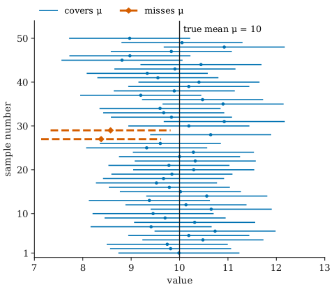
Fifty horizontal interval segments stacked vertically, with a vertical line at the true mean of 10. Forty-eight intervals cross the line; two, drawn thicker, dashed and in a different colour, lie entirely to its left. — Fifty 95% confidence intervals, each computed from its own simulated sample of n = 10 values from a normal population with μ = 10 and known σ = 2, using x̄ ± 1.96 σ/√n. In this simulation 48 intervals contain μ and 2 miss it (dashed, with diamond markers); in the long run about 5%, or 2.5 in 50, would miss.

Every interval has the same width here because $\sigma$ is known; only the centre $\bar{x}$ moves from sample to sample. Most intervals cover $\mu$ ; a few, from samples whose means happened to land far from $\mu$ , do not. Nothing in the data of a single sample tells you which kind of interval you have.

The z-interval: a mean with known standard deviation

Let $x_1, \dots, x_n$ be a random sample from a population with unknown mean $\mu$ and known standard deviation $\sigma$ . Assume either that the population is normal or that $n$ is large enough for the central limit theorem to apply. Then the sample mean $\bar{X}$ is approximately normal with mean $\mu$ and standard error $\sigma/\sqrt{n}$ , so the standardized mean

Z = \frac{\bar{X} - \mu}{\sigma / \sqrt{n}}

has a standard normal distribution. Since $P(-1.96 \le Z \le 1.96) \approx 0.95$ , we can write

P\!\left(-1.96 \le \frac{\bar{X} - \mu}{\sigma/\sqrt{n}} \le 1.96\right) \approx 0.95.

Multiplying through by $\sigma/\sqrt{n}$ and rearranging the inequalities to isolate $\mu$ gives the same event in a different form:

P\!\left(\bar{X} - 1.96\frac{\sigma}{\sqrt{n}} \le \mu \le \bar{X} + 1.96\frac{\sigma}{\sqrt{n}}\right) \approx 0.95.

Read this carefully: $\mu$ is a fixed number, and the endpoints are random because $\bar{X}$ is. The statement is about the random interval capturing the fixed $\mu$ . Plugging in the observed $\bar{x}$ gives the 95% z-interval

\bar{x} \pm z^* \frac{\sigma}{\sqrt{n}},

where the critical value $z^* = 1.96$ for 95% confidence. For other confidence levels, $z^*$ is chosen so that the central area under the standard normal density between $-z^*$ and $z^*$ equals the confidence level: $z^* \approx 1.645$ for 90% and $z^* \approx 2.576$ for 99%. The quantity $z^* \sigma/\sqrt{n}$ is called the margin of error.

The t-interval: a mean with unknown standard deviation

In practice $\sigma$ is almost never known, so we replace it by the sample standard deviation $s$ . This adds uncertainty, because $s$ itself varies from sample to sample. To account for it, the critical value comes from the $t$ distribution with $n - 1$ degrees of freedom instead of the standard normal. The $t$ distribution is bell-shaped and centred at zero like the standard normal, but has heavier tails, so its critical values are larger. The t-interval is

\bar{x} \pm t^* \frac{s}{\sqrt{n}},

where $t^*$ cuts off an area of 2.5% in each tail of the $t$ distribution with $n-1$ degrees of freedom (for 95% confidence). For $n = 16$ , $t^* \approx 2.131$ compared with $1.96$ ; as $n$ grows, $t^*$ approaches $1.96$ . The t-interval is exact when the population is normal and is a good approximation for moderately non-normal populations when $n$ is not small. For strongly skewed data and small $n$ it can be unreliable.

The interval for a proportion

If $k$ of $n$ independent trials are successes, the sample proportion $\hat{p} = k/n$ estimates the population proportion $p$ . Its standard error is $\sqrt{p(1-p)/n}$ , which we estimate by plugging in $\hat p$ . The resulting Wald interval is

\hat{p} \pm z^* \sqrt{\frac{\hat{p}(1 - \hat{p})}{n}}.

It relies on the normal approximation to the binomial distribution and works well when there are plenty of both successes and failures (a common rule of thumb asks for at least 10 of each). It performs poorly for small $n$ or for $p$ near $0$ or $1$ : its actual coverage can be well below the nominal 95%. In the extreme case of $0$ successes in $20$ trials it gives the interval from $0$ to $0$ , claiming complete certainty. Better-behaved alternatives such as the Wilson interval are preferred in those situations.

Worked example

A manufacturer tests $n = 16$ batteries and records their lifetimes. The sample mean is $\bar{x} = 23.4$ hours and the sample standard deviation is $s = 3.2$ hours. Lifetimes in this kind of test are roughly normal. Find a 95% confidence interval for the mean lifetime $\mu$ of all batteries of this type.

Step 1: estimated standard error.

\frac{s}{\sqrt{n}} = \frac{3.2}{\sqrt{16}} = 0.8 \text{ hours}.

Step 2: critical value. With $n - 1 = 15$ degrees of freedom, the 97.5th percentile of the $t$ distribution is $t^* \approx 2.131$ (from a table or software, for example scipy.stats.t.ppf(0.975, 15)).

Step 3: margin of error. $2.131 \times 0.8 \approx 1.705$ hours.

Step 4: interval.

23.4 \pm 1.705, \quad \text{that is, from about } 21.7 \text{ to } 25.1 \text{ hours}.

Using $1.96$ instead of $2.131$ would give the narrower interval 21.8 to 25.0 hours, which overstates the precision because it ignores the uncertainty in $s$ . A 99% interval uses $t^* \approx 2.947$ and is wider: about 21.0 to 25.8 hours.

A proportion. In a survey, 540 of 1000 randomly chosen people support a proposal. Then $\hat p = 0.54$ , the estimated standard error is $\sqrt{0.54 \times 0.46 / 1000} \approx 0.0158$ , and the 95% Wald interval is $0.54 \pm 1.96 \times 0.0158$ , or about $0.509$ to $0.571$ . Here there are hundreds of successes and failures, so the Wald interval is reliable.

What makes an interval wider or narrower

The margin of error is (critical value) × (standard deviation) / $\sqrt{n}$ , so three things control the width:

Confidence level. Higher confidence needs a larger critical value and a wider interval. A 100% interval would have to include every possible value and would be useless.
Variability in the population. A larger $\sigma$ (or $s$ ) gives a wider interval.
Sample size. The width shrinks in proportion to $1/\sqrt{n}$ . Quadrupling the sample size halves the width.

Interpreting a confidence interval

This is the part people most often get wrong.

In the frequentist framework used here, the parameter $\mu$ is a fixed, unknown number; it is not random. The 95% describes the procedure: if you repeated the whole study many times, computing a new interval each time, about 95% of those intervals would contain $\mu$ . This long-run fraction is called the coverage of the procedure.

Once you have computed a specific interval, such as 21.7 to 25.1 hours, it either contains $\mu$ or it does not. In this framework it is not correct to say “there is a 95% probability that $\mu$ lies between 21.7 and 25.1”. A correct phrasing is: “we are 95% confident that the interval from 21.7 to 25.1 hours contains the mean lifetime”, where “95% confident” is shorthand for “this interval was produced by a method that succeeds 95% of the time”.

Bayesian credible intervals do make direct probability statements about a parameter, but they require a prior distribution and answer a different question.

Confidence intervals are closely tied to hypothesis testing: for the z- and t-intervals above, the 95% interval contains exactly those values of the mean that the matching two-sided test at the 5% significance level would not reject.

Common misunderstandings

“There is a 95% chance the true mean is in this interval.” In the frequentist sense, no: the 95% refers to the long-run success rate of the procedure, not to one computed interval; see above.

“95% of the data lie inside the interval.” A confidence interval for a mean describes uncertainty about the mean, not the spread of individual values. With $n = 16$ batteries, the interval for $\mu$ is about 3.4 hours wide, while individual lifetimes vary with standard deviation 3.2 hours, so many batteries fall outside it. As $n$ grows the interval shrinks toward a point; the spread of the data does not.

“The interval accounts for all sources of error.” It accounts only for random sampling variability under the assumed model. A biased sample, measurement error, or a wrong model can make an interval confidently wrong.

“Overlapping intervals mean no significant difference.” Two 95% intervals can overlap somewhat even when a test comparing the two means finds a significant difference. To compare two groups, compute an interval for the difference directly.