Likelihood and Maximum Likelihood Estimation

The likelihood measures how well each parameter value explains the observed data; the maximum likelihood estimate is the value that explains them best.

Prerequisites: Point Estimation, Random Variables, Bernoulli and Binomial Distributions.

The likelihood of a parameter value is the probability (or probability density) that a model with that parameter value assigns to the data you actually observed. Maximum likelihood estimation picks, as the estimate of the parameter, the value under which the observed data would have been most probable.

It is the most widely used general recipe for building estimators. Given almost any probability model, from a coin toss to logistic regression, maximum likelihood tells you how to turn data into parameter estimates, and in large samples those estimates are usually as precise as any reasonable alternative.

Intuition

You toss a coin 10 times and see 7 heads. What is a sensible guess for $p$, the probability of heads?

Try a few candidate values and ask how likely the observed result would be under each:

• if $p = 0.5$, getting exactly 7 heads has probability about $0.117$;
• if $p = 0.7$, it has probability about $0.267$;
• if $p = 0.9$, it has probability about $0.057$.

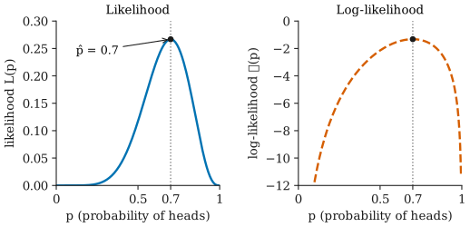
The data are more than twice as probable under $p = 0.7$ as under a fair coin, and much more probable than under $p = 0.9$. Maximum likelihood formalizes this comparison: compute that probability for every candidate $p$, and choose the $p$ that makes it largest.

The likelihood function

Suppose the data $x_1, \dots, x_n$ are modelled as observations of random variables whose distribution depends on an unknown parameter $\theta$. Write $p(x \mid \theta)$ for the probability mass function of a discrete observation, or $f(x \mid \theta)$ for the density of a continuous one. If the observations are independent, the joint probability (or density) of the whole data set is the product of the individual ones.

The likelihood function is that same expression, read as a function of $\theta$ with the data held fixed:

$$L(\theta) = \prod_{i=1}^n p(x_i \mid \theta) \quad \text{(discrete)}, \qquad L(\theta) = \prod_{i=1}^n f(x_i \mid \theta) \quad \text{(continuous)}.$$

The formula is identical to the probability model. What changes is the question. The model asks, “for a fixed $\theta$, how probable are different data sets?” The likelihood asks, “for these fixed data, how well does each $\theta$ explain them?”

The likelihood is not a probability distribution for the parameter

$L(\theta)$ is not the probability that $\theta$ is the true value. It is a probability of the data, evaluated at many different values of $\theta$. Nothing forces it to add or integrate to $1$ over $\theta$. For the coin example,

$$\int_0^1 \binom{10}{7} p^7 (1-p)^3 \, dp = \frac{1}{11} \approx 0.091,$$

not $1$. Only ratios of likelihoods are meaningful: $L(0.7)/L(0.5) \approx 2.28$ says the data are about 2.3 times as probable if $p = 0.7$ as if $p = 0.5$. Turning this into a probability statement about $p$ itself requires a prior distribution and Bayes’ theorem, which is a different approach to inference.

The log-likelihood

In practice we almost always work with the log-likelihood

$$\ell(\theta) = \log L(\theta) = \sum_{i=1}^n \log p(x_i \mid \theta),$$

(with $f$ in place of $p$ for continuous data). There are three reasons:

• the logarithm turns a product into a sum, which is much easier to differentiate;
• a product of many probabilities smaller than $1$ quickly becomes too small for a computer to store, while a sum of logarithms does not;
• $\log$ is strictly increasing, so $\ell(\theta)$ and $L(\theta)$ are largest at exactly the same $\theta$. Nothing is lost by switching.

Maximum likelihood estimation

The maximum likelihood estimate (MLE) of $\theta$ is the value that maximizes the likelihood:

$$\hat{\theta} = \arg\max_{\theta} L(\theta) = \arg\max_{\theta} \ell(\theta).$$

Here $\arg\max$ means “the value of $\theta$ at which the maximum is attained”. When $\ell$ is smooth and the maximum is not at the edge of the allowed parameter values, it can usually be found by setting the derivative to zero, $\ell'(\theta) = 0$, and checking that this point is a maximum (for example, that $\ell''(\hat\theta) < 0$). When no closed-form solution exists, as in logistic regression, the maximum is found numerically.

Worked example: a coin

We observe $k = 7$ heads in $n = 10$ independent tosses. The number of heads follows a binomial distribution with parameter $p$, where $0 < p < 1$.

Step 1: write the likelihood. The binomial PMF evaluated at the observed $k$, viewed as a function of $p$:

$$L(p) = \binom{n}{k} p^k (1-p)^{n-k} = \binom{10}{7} p^7 (1-p)^3.$$

Step 2: take logarithms.

$$\ell(p) = \log\binom{n}{k} + k \log p + (n-k)\log(1-p).$$

The first term does not depend on $p$, so it does not affect where the maximum is.

Step 3: differentiate and set to zero.

$$\ell'(p) = \frac{k}{p} - \frac{n-k}{1-p} = 0.$$

Multiplying both sides by $p(1-p)$ gives $k(1-p) = (n-k)p$, which simplifies to $k = np$. So

$$\hat{p} = \frac{k}{n} = \frac{7}{10} = 0.7.$$

Step 4: check that it is a maximum. The second derivative $\ell''(p) = -k/p^2 - (n-k)/(1-p)^2$ is negative for every $p$ between $0$ and $1$, so $\ell$ is concave and $p = 0.7$ is its single maximum. This matches the peak in the figure.

The answer, “the proportion of heads you observed”, is what intuition suggests. The value of the method is that the same four steps work for models where intuition gives no obvious answer. One edge case: if $k = 0$ or $k = n$, the likelihood is largest at the boundary, giving $\hat p = 0$ or $\hat p = 1$, which is a poor estimate from a small sample.

A continuous example: waiting times

Five waiting times, in minutes, are modelled as independent draws from an exponential distribution with rate $\lambda > 0$, whose density is $f(x \mid \lambda) = \lambda e^{-\lambda x}$ for $x \ge 0$. The data are $2.0, 0.5, 4.1, 1.3, 2.6$.

The likelihood is a product of densities:

$$L(\lambda) = \prod_{i=1}^n \lambda e^{-\lambda x_i} = \lambda^n \exp\!\left(-\lambda \sum_{i=1}^n x_i\right),$$

so $\ell(\lambda) = n \log \lambda - \lambda \sum_{i=1}^n x_i$. Setting $\ell'(\lambda) = n/\lambda - \sum x_i = 0$ gives

$$\hat{\lambda} = \frac{n}{\sum_{i=1}^n x_i} = \frac{1}{\bar{x}}.$$

Here $\sum x_i = 10.5$ and $\bar{x} = 2.1$ minutes, so $\hat{\lambda} = 1/2.1 \approx 0.476$ per minute. Since $\ell''(\lambda) = -n/\lambda^2 < 0$, this is a maximum.

The same reasoning applied to a normal sample with unknown mean $\mu$ shows that the MLE of $\mu$ is the sample mean $\bar{x}$: the log-likelihood is, apart from constants, $-\sum (x_i - \mu)^2 / (2\sigma^2)$, which is largest when $\mu$ minimizes the sum of squared distances to the data, and that is $\mu = \bar{x}$.

Properties of maximum likelihood estimators

Under standard regularity conditions (roughly: the model is correct, the number of parameters stays fixed as $n$ grows, the true value is not on the boundary of the allowed values, and the likelihood is smooth), maximum likelihood estimators have attractive large-sample properties.

• Consistency. As the sample size grows, $\hat\theta$ gets arbitrarily close to the true $\theta$ with probability approaching $1$.
• Asymptotic normality. For large $n$, the sampling distribution of $\hat\theta$ is approximately normal, centred at the true $\theta$. Its standard deviation can be estimated from how sharply curved the log-likelihood is at its peak: a sharp peak means a precise estimate. For the coin, this gives the familiar standard error $\sqrt{\hat p(1-\hat p)/n}$, used to build confidence intervals.
• Efficiency. In large samples, no other well-behaved estimator has a smaller variance.
• Invariance. If $\hat\theta$ is the MLE of $\theta$, then $g(\hat\theta)$ is the MLE of $g(\theta)$ for any function $g$. In the waiting-time example, the MLE of the mean waiting time $1/\lambda$ is $1/\hat\lambda = \bar{x} = 2.1$ minutes.

These are statements about large samples. In small samples, an MLE can be noticeably biased. The standard example is the variance of a normal distribution: its MLE is

$$\hat{\sigma}^2 = \frac{1}{n} \sum_{i=1}^n (x_i - \bar{x})^2,$$

with $n$ rather than $n - 1$ in the denominator. On average it underestimates $\sigma^2$ by the factor $(n-1)/n$, for example by 20% when $n = 5$. That is why the usual sample variance divides by $n - 1$. The bias vanishes as $n$ grows, consistent with the large-sample properties above.

Common misunderstandings

“The likelihood is the probability that the parameter is correct.” It is the probability (or density) of the observed data under that parameter value. It does not sum or integrate to $1$ over the parameter, and it says nothing about which parameter values were plausible before seeing the data.

“Likelihood and probability are the same word.” In everyday speech they are. In statistics, probability describes possible data for a fixed parameter; likelihood compares parameter values for fixed data.

“The MLE is the true value.” It is an estimate, and it varies from sample to sample like any other statistic. With 7 heads in 10 tosses, $\hat p = 0.7$, but a fair coin produces 7 or more heads in 10 tosses about 17% of the time.

“Maximum likelihood always gives the best estimator.” Its optimality is a large-sample result that assumes the model is correct. With small samples, many parameters, or a misspecified model, it can be biased or unstable, and other estimators may do better.

Further reading

• Larry Wasserman, All of Statistics: A Concise Course in Statistical Inference, Springer, 2004. Covers maximum likelihood and its large-sample theory concisely.
• George Casella and Roger L. Berger, Statistical Inference, 2nd ed., Duxbury, 2002. A rigorous treatment of likelihood, including the invariance property and regularity conditions.

Related articles

• Confidence Intervals — A range of plausible values for a parameter, produced by a procedure that captures the true value in a stated fraction of repeated samples.
• Exponential Distribution — The distribution of the waiting time until the next event when events occur independently at a constant average rate.
• Bayes' Theorem — A rule for reversing a conditional probability, turning P(evidence | hypothesis) into P(hypothesis | evidence).
• Sampling Distributions — The distribution of a statistic, such as the sample mean, over all the samples that could have been drawn.