Bayes' Theorem

A rule for reversing a conditional probability, turning P(evidence | hypothesis) into P(hypothesis | evidence).

Prerequisites: Conditional Probability.

Bayes’ theorem is a formula for turning one conditional probability around: from the probability of the evidence given a hypothesis, $P(B \mid A)$, it computes the probability of the hypothesis given the evidence, $P(A \mid B)$. It is the mathematical rule for updating a belief when new information arrives, and it explains why a positive result from a fairly accurate medical test can still leave the disease unlikely.

Intuition

A test for a disease is described by how it behaves in people whose status is known: how often it is positive for people who have the disease, and how often for people who do not. A patient, however, wants the reverse: given a positive result, how likely is it that I have the disease?

These two questions have different answers, and the gap between them depends on how common the disease is in the first place. If a disease is rare, even a small false-positive rate among the many healthy people can produce more positive results than the disease itself does among the few sick people. Bayes’ theorem keeps track of both sources of positive results and weighs them correctly.

Derivation

Bayes’ theorem follows in two lines from the definition of conditional probability. For events $A$ and $B$ with $P(A) > 0$ and $P(B) > 0$, the multiplication rule gives the probability of “both $A$ and $B$” in two ways:

$$P(A \cap B) = P(A \mid B)\, P(B) = P(B \mid A)\, P(A).$$

Dividing the two right-hand expressions by $P(B)$ gives Bayes’ theorem:

$$P(A \mid B) = \frac{P(B \mid A)\, P(A)}{P(B)}.$$

The denominator $P(B)$ is usually not known directly. The law of total probability computes it by splitting into the cases “$A$” and “not $A$”:

$$P(B) = P(B \mid A)\,P(A) + P(B \mid A^c)\,P(A^c).$$

Substituting gives the form most often used in practice:

$$P(A \mid B) = \frac{P(B \mid A)\,P(A)}{P(B \mid A)\,P(A) + P(B \mid A^c)\,P(A^c)}.$$

More generally, if $A_1, \dots, A_k$ are mutually exclusive hypotheses, exactly one of which is true, then

$$P(A_j \mid B) = \frac{P(B \mid A_j)\,P(A_j)}{\sum_{i=1}^k P(B \mid A_i)\,P(A_i)}.$$

Prior, likelihood, and posterior

When $A$ is a hypothesis and $B$ is observed evidence, each piece of the formula has a name:

• $P(A)$ is the prior probability: how plausible $A$ was before seeing the evidence.
• $P(B \mid A)$ is the likelihood: how probable the observed evidence is if $A$ is true.
• $P(A \mid B)$ is the posterior probability: how plausible $A$ is after seeing the evidence.
• $P(B)$ is the overall probability of the evidence, which makes the posterior probabilities of all hypotheses add up to 1.

Read this way, Bayes’ theorem says: posterior is proportional to likelihood times prior. Evidence raises the probability of hypotheses that predicted it well and lowers the probability of hypotheses that predicted it poorly. The word “likelihood” here is related to, but not the same as, the likelihood function used in estimation.

Worked example: a medical test

A condition affects 1% of a population. A screening test for it has these properties:

• Sensitivity 90%: among people who have the condition, 90% test positive.
• False-positive rate 9%: among people who do not have the condition, 9% test positive. (Equivalently, the specificity, the proportion of healthy people who test negative, is 91%.)

A randomly chosen person tests positive. What is the probability that they have the condition?

Let $D$ be “has the condition” and $+$ be “tests positive”. We know

$$P(D) = 0.01, \qquad P(+ \mid D) = 0.90, \qquad P(+ \mid D^c) = 0.09.$$

Step 1: the probability of a positive test. By the law of total probability,

$$P(+) = 0.90 \times 0.01 + 0.09 \times 0.99 = 0.0090 + 0.0891 = 0.0981.$$

Step 2: Bayes’ theorem.

$$P(D \mid +) = \frac{P(+ \mid D)\,P(D)}{P(+)} = \frac{0.0090}{0.0981} \approx 0.092.$$

Despite the test detecting 90% of cases, a positive result means only about a 9.2% chance of having the condition. More than 90% of positive results are false alarms.

The same calculation with natural frequencies

The result is easier to believe when probabilities are replaced by counts of people. Imagine 10,000 people tested.

• 1% of them, 100 people, have the condition. The test is positive for 90% of these: 90 true positives, and 10 are missed.
• The other 9,900 people do not have the condition. The test is positive for 9% of these: 891 false positives, and 9,009 correctly test negative.

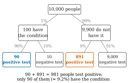
Altogether $90 + 891 = 981$ people test positive, and only 90 of them have the condition:

$$P(D \mid +) = \frac{90}{981} \approx 0.092.$$

The reason is now visible: the false-positive rate is small, but it applies to a very large group. Nine percent of 9,900 healthy people is far more than 90% of 100 sick people.

What a negative result means

The same tree answers other questions. Of the $10 + 9{,}009 = 9{,}019$ people who test negative, only 10 have the condition, so $P(D \mid -) = 10/9{,}019 \approx 0.0011$. A negative result is very reassuring, because the condition was rare to begin with.

Updating twice

Suppose the person who tested positive takes the test again, and assume the two results are independent given the person’s true status. The posterior from the first test, about $0.092$, becomes the prior for the second. Of the 981 positives, about $0.90 \times 90 = 81$ sick and $0.09 \times 891 \approx 80$ healthy people would test positive again, so

$$P(D \mid \text{two positives}) \approx \frac{81}{81 + 80.19} \approx 0.50.$$

Two positive results raise the probability to about one half. (In practice, repeated tests on the same person are often not independent, so a different, confirmatory test is usually used.)

Common misunderstandings

The base-rate fallacy. Ignoring the prior $P(A)$, here the 1% prevalence, and judging the posterior from the test’s accuracy alone. The 90% sensitivity tempts people to answer “about 90%”, but the correct answer is about 9%. Whenever a condition is rare, the base rate matters a great deal.

“P(positive | disease) is the same as P(disease | positive).” These are conditional probabilities in opposite directions. They can be very different, as the example shows. Confusing them is also known as the prosecutor’s fallacy when it appears in court: the probability of the evidence given innocence is not the probability of innocence given the evidence.

“Bayes’ theorem is only for Bayesian statistics.” The theorem itself is an uncontroversial consequence of the definition of conditional probability, accepted by every school of statistics. What is debated is whether it is appropriate to put prior probabilities on unknown parameters, which is the starting point of Bayesian inference.

“A p-value is the probability that the null hypothesis is true.” A p-value is computed assuming the null hypothesis is true, so it is a probability of data given a hypothesis, not of a hypothesis given data. Turning one into the other would require Bayes’ theorem and a prior.

Further reading

• Joseph K. Blitzstein and Jessica Hwang, Introduction to Probability, 2nd ed., CRC Press, 2019. Develops Bayes’ rule alongside conditional probability, with many testing examples.
• David M. Diez, Mine Çetinkaya-Rundel, and Christopher D. Barr, OpenIntro Statistics, 4th ed., 2019. Free online; uses tree diagrams to apply Bayes’ theorem.

Related articles

• Statistical Independence — Two events are independent when knowing that one happened does not change the probability of the other.
• Likelihood and Maximum Likelihood Estimation — The likelihood measures how well each parameter value explains the observed data; the maximum likelihood estimate is the value that explains them best.
• P-values and Statistical Significance — The probability, assuming the null hypothesis and the model are true, of a result at least as extreme as the one observed.