Random Variables

A random variable assigns a number to each outcome of a random experiment; its distribution is described by a PMF, a PDF, or a CDF.

Prerequisites: Introduction to Probability.

A random variable is a numerical quantity whose value depends on the outcome of a random experiment: the number of heads in ten coin tosses, the sum of two dice, a person’s height, the time until the next bus. Random variables let us use ordinary arithmetic and algebra (sums, averages, functions) on uncertain quantities, and they are the objects that statistical models are built from.

Intuition

The outcomes of an experiment are not always numbers. Tossing a coin three times produces sequences like HTH. But we usually care about a number computed from the outcome, such as “how many heads”. That rule (take an outcome, return a number) is a random variable.

The name is a little misleading: a random variable is not a variable in the algebra sense, and the function itself is not random. The randomness is in which outcome occurs; once the outcome is known, the value of the random variable is determined.

Definition

A random variable $X$ is a function that assigns a real number $X(\omega)$ to each outcome $\omega$ in the sample space $\Omega$ .

Random variables are written with capital letters ( $X$ , $Y$ , $S$ ), and particular values they can take with lower-case letters ( $x$ , $y$ , $s$ ). Statements such as “ $X = 2$ ” or “ $X \le x$ ” describe events, namely the set of outcomes for which they are true, so they have probabilities.

Example. Toss a coin three times and let $X$ be the number of heads. Then $X(\text{HHH}) = 3$ , $X(\text{HTH}) = 2$ , $X(\text{TTT}) = 0$ , and so on. The event $\{X = 2\}$ is the set $\{\text{HHT}, \text{HTH}, \text{THH}\}$ , and for a fair coin $P(X = 2) = 3/8$ .

The distribution of a random variable is the complete description of which values it can take and how probable they are. Two kinds of random variable need slightly different tools.

Discrete random variables and the PMF

A random variable is discrete if it can take only a finite or countable list of values, such as $0, 1, 2, \dots$ . Counts are typical examples.

The distribution of a discrete random variable is given by its probability mass function (PMF):

p(x) = P(X = x).

Each $p(x)$ is an actual probability, so a PMF satisfies

p(x) \ge 0 \quad \text{for all } x, \qquad \sum_x p(x) = 1,

where the sum runs over all values $X$ can take. The probability that $X$ lands in a set of values is the sum of the masses on those values.

Continuous random variables and the PDF

A random variable is continuous if it can take any value in an interval, and the probability of every single exact value is zero. Measurements such as times, lengths, and weights are typically modelled this way.

Because single values have probability zero, a PMF is useless here. Instead the distribution is described by a probability density function (PDF) $f(x)$ , and probabilities are areas under it:

P(a \le X \le b) = \int_a^b f(x)\, dx.

A PDF satisfies $f(x) \ge 0$ and $\int_{-\infty}^{\infty} f(x)\,dx = 1$ .

The value $f(x)$ is a density, not a probability. It can be larger than 1; only the area under $f$ over an interval is a probability. Roughly, for a small interval of width $\Delta x$ around $x$ , $P(x \le X \le x + \Delta x) \approx f(x)\,\Delta x$ .

Example. If a bus arrives at a uniformly random time within the next 10 minutes, the waiting time $X$ (in minutes) has density $f(x) = 1/10$ for $0 \le x \le 10$ and $0$ elsewhere. The probability of waiting at most 3 minutes is the area of a rectangle of width 3 and height $1/10$ , which is $0.3$ . The probability of waiting exactly 3 minutes is $0$ . This is the uniform distribution.

The cumulative distribution function

One tool works for every random variable, discrete or continuous: the cumulative distribution function (CDF),

F(x) = P(X \le x).

It gives the probability that $X$ is at most $x$ . Every CDF starts near 0 for very small $x$ , never decreases, and approaches 1 for large $x$ . Probabilities of intervals follow by subtraction: $P(a < X \le b) = F(b) - F(a)$ .

The CDF is connected to the other descriptions:

For a discrete variable, $F(x)$ is the sum of $p(t)$ over all values $t \le x$ , and its graph is a staircase that jumps by $p(x)$ at each possible value $x$ .
For a continuous variable, $F(x) = \int_{-\infty}^x f(t)\,dt$ is the area to the left of $x$ , and the density is the derivative of the CDF, $f(x) = F'(x)$ . In the bus example, $F(x) = x/10$ for $0 \le x \le 10$ .

The article on probability distributions compares PMFs, PDFs, and CDFs side by side.

Worked example: the sum of two dice

Roll two fair six-sided dice and let $S$ be the sum of the two faces.

Step 1: the sample space. An outcome is an ordered pair (first die, second die), such as $(2, 5)$ . There are $6 \times 6 = 36$ outcomes, all equally likely, each with probability $1/36$ .

Step 2: the values of S. The sum ranges from $2$ , from $(1, 1)$ , to $12$ , from $(6, 6)$ . So $S$ is a discrete random variable with eleven possible values.

Step 3: count the outcomes for each value. A sum of 7 arises from $(1,6), (2,5), (3,4), (4,3), (5,2), (6,1)$ : six outcomes. A sum of 2 arises only from $(1,1)$ . In general, the number of outcomes giving sum $s$ is $6 - |s - 7|$ , so the PMF is

p(s) = P(S = s) = \frac{6 - |s - 7|}{36}, \qquad s = 2, 3, \dots, 12.

Eleven vertical stems at sums 2 through 12. Their heights rise steadily from 1/36 at a sum of 2 to a peak of 6/36 at 7, then fall back to 1/36 at 12, forming a symmetric triangle. — PMF of the sum S of two fair dice. Each stem is a probability P(S = s), shown as a fraction of the 36 equally likely outcomes. The stems add up to 1.

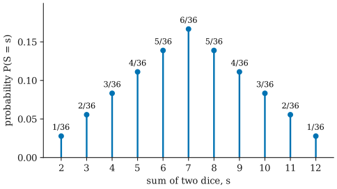
Step 4: use the PMF. Because the stems are probabilities, we can add them:

$P(S = 7) = 6/36 = 1/6$ , the most likely sum.
$P(S \ge 10) = (3 + 2 + 1)/36 = 6/36 = 1/6$ .
The CDF at 4 is $F(4) = P(S \le 4) = (1 + 2 + 3)/36 = 6/36 = 1/6$ .
The masses add to one: $(1 + 2 + 3 + 4 + 5 + 6 + 5 + 4 + 3 + 2 + 1)/36 = 36/36 = 1$ .

The example also shows why the counting rule from the introduction to probability must be applied to the right sample space: the 36 ordered pairs are equally likely, but the 11 sums are not.

Summaries of a random variable

A distribution contains all the information about a random variable, but it is often useful to summarize it with a few numbers. The two most important are:

the expected value $\E[X]$ , the long-run average value, which for the sum of two dice is $7$ ;
the variance $\Var(X)$ , which measures how spread out the values are around the expected value.

Two random variables can also be related to each other. When knowing the value of one tells us nothing about the other, they are independent.

Common misunderstandings

“A random variable is a random number.” It is a function from outcomes to numbers. The same experiment can carry many random variables: from two dice we can define the sum, the maximum, the difference, and so on.

“The PDF value is the probability of that value.” For a continuous variable, $f(x)$ is a density and $P(X = x) = 0$ . Only areas under $f$ are probabilities.

“A PMF can be drawn as a smooth curve.” A discrete variable puts probability only on separate points; there is no probability between them. Draw a PMF with stems or bars, not a continuous line.

“X and x are interchangeable.” $X$ is the random variable; $x$ is a fixed number. $P(X = x)$ asks how likely the random quantity is to equal that particular number.