Uniform Distribution

The distribution that spreads probability evenly, either over an interval or over a finite set of equally likely values.

Prerequisites: Probability Distributions, Expected Value, Variance of a Random Variable.

The uniform distribution spreads probability evenly. In its continuous form, every stretch of the same length inside an interval from $a$ to $b$ is equally likely to contain the value, and values outside the interval are impossible. In its discrete form, each of a finite set of values, such as the six faces of a fair die, has the same probability.

It is the simplest model of “no value is favoured over any other” and is mostly useful for that reason: as a model of complete uncertainty within known limits, as a building block in probability arguments, and as the starting point of almost every computer simulation, since random number generators produce (approximately) uniform numbers between $0$ and $1$ .

Intuition

Suppose a bus comes every 20 minutes and you arrive at the stop at a random moment, without checking the timetable. Your waiting time could be anything from $0$ to $20$ minutes, and there is no reason for any part of that range to be more likely than another. The chance of waiting between 0 and 5 minutes is the same as the chance of waiting between 15 and 20 minutes: each stretch is a quarter of the window, so each has probability $0.25$ .

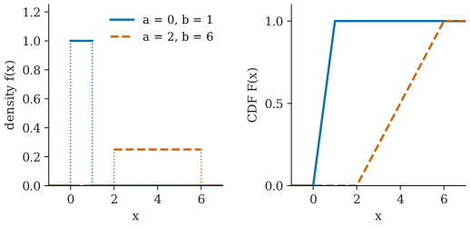
That is the continuous uniform distribution: probability is proportional to length. Its density is flat, like a rectangle, and the height of the rectangle is whatever makes its area equal to $1$ .

Left: two flat, rectangular densities. The one on the interval from 0 to 1 has height 1; the wider one from 2 to 6 has height 0.25, so both rectangles have area 1. Right: the corresponding CDFs are 0 to the left of the interval, rise in a straight line across it, and stay at 1 to the right. — Continuous uniform distributions on [0, 1] (solid) and [2, 6] (dashed). Left: densities; a wider interval gives a lower rectangle. Dotted lines mark the jumps at the ends of each interval. Right: the CDF rises linearly from 0 at a to 1 at b.

Definition

A continuous random variable $X$ has a uniform distribution on the interval from $a$ to $b$ , written $X \sim \text{Uniform}(a, b)$ , if its probability density function is

f(x) = \begin{cases} \dfrac{1}{b - a} & \text{if } a \le x \le b, \\[1ex] 0 & \text{otherwise.} \end{cases}

The two parameters are the endpoints $a$ and $b$ , any real numbers with $a < b$ . The height $1/(b-a)$ is fixed by the requirement that the total area is $1$ : a rectangle of width $b - a$ and height $1/(b-a)$ has area exactly $1$ . The special case $\text{Uniform}(0, 1)$ is called the standard uniform distribution.

Whether the endpoints are included makes no difference, because a single point has probability $0$ for a continuous variable.

Probabilities are lengths

For any interval $[c, d]$ inside $[a, b]$ ,

P(c \le X \le d) = \frac{d - c}{b - a},

the length of the interval divided by the length of the whole range. The cumulative distribution function is

F(x) = P(X \le x) = \begin{cases} 0 & \text{if } x < a, \\[0.5ex] \dfrac{x - a}{b - a} & \text{if } a \le x \le b, \\[1ex] 1 & \text{if } x > b, \end{cases}

a straight ramp from $0$ to $1$ across the interval, as in the right panel of the figure.

Mean and variance

If $X \sim \text{Uniform}(a, b)$ , then

\E[X] = \frac{a + b}{2}, \qquad \Var(X) = \frac{(b - a)^2}{12}.

The mean is the midpoint of the interval, as symmetry suggests. It also follows from the integral:

\E[X] = \int_a^b \frac{x}{b - a}\, dx = \frac{b^2 - a^2}{2(b - a)} = \frac{a + b}{2},

using $b^2 - a^2 = (b - a)(b + a)$ . For the variance, first compute

\E[X^2] = \int_a^b \frac{x^2}{b - a}\, dx = \frac{b^3 - a^3}{3(b - a)} = \frac{a^2 + ab + b^2}{3},

using $b^3 - a^3 = (b - a)(a^2 + ab + b^2)$ . Then

\Var(X) = \E[X^2] - (\E[X])^2 = \frac{a^2 + ab + b^2}{3} - \frac{(a + b)^2}{4} = \frac{(b - a)^2}{12}.

(Put both fractions over $12$ : the numerator is $4a^2 + 4ab + 4b^2 - 3a^2 - 6ab - 3b^2 = (b - a)^2$ .)

So the variance depends only on the width of the interval, not on where it sits, and the standard deviation is $(b - a)/\sqrt{12} \approx 0.29\,(b - a)$ . For the standard uniform, $\Var(X) = 1/12 \approx 0.083$ .

How the shape depends on a and b

There is only one shape, a rectangle; the parameters move and stretch it.

Shifting $a$ and $b$ by the same amount moves the rectangle without changing it, just as changing the mean of a normal distribution moves its bell curve.
Widening the interval makes the rectangle lower, since the area must stay $1$ . A narrow interval gives a tall rectangle, and the density can exceed $1$ : $\text{Uniform}(0, 0.5)$ has density $2$ on its interval.

Worked example

A bus arrives every 20 minutes and you turn up at a random time, so your waiting time $W$ in minutes is $\text{Uniform}(0, 20)$ , with density $1/20$ on that interval.

Step 1: average wait. $\E[W] = (0 + 20)/2 = 10$ minutes.

Step 2: a long wait. The probability of waiting more than 15 minutes is the length from 15 to 20 divided by 20:

P(W > 15) = \frac{20 - 15}{20} = 0.25.

Step 3: a range. The probability of waiting between 5 and 8 minutes is $(8 - 5)/20 = 0.15$ .

Step 4: spread. $\Var(W) = 20^2 / 12 \approx 33.3$ square minutes, so the standard deviation is $20/\sqrt{12} \approx 5.8$ minutes. A typical wait is about 6 minutes away from the 10-minute average, which fits a range that runs evenly from 0 to 20.

The discrete uniform distribution

A discrete uniform distribution puts equal probability on each of a finite set of values. The roll of a fair six-sided die is the standard example: $P(X = k) = 1/6$ for $k = 1, 2, \dots, 6$ .

It differs from the continuous version in the usual way that discrete and continuous distributions differ: each possible value has a positive probability, $1/6$ , rather than a density, and probabilities of sets are sums rather than areas. The mean is again the midpoint, $(1 + 6)/2 = 3.5$ , but the variance is not $(b - a)^2/12$ . For the die,

\Var(X) = \E[X^2] - (\E[X])^2 = \frac{1 + 4 + 9 + 16 + 25 + 36}{6} - 3.5^2 = \frac{91}{6} - 12.25 = \frac{35}{12} \approx 2.92,

whereas the continuous formula with $a = 1$ and $b = 6$ would give $25/12 \approx 2.08$ .

Uniform numbers in simulation

Computers generate pseudo-random numbers that behave like independent draws from $\text{Uniform}(0, 1)$ . Almost every other random quantity in a simulation is built from these.

Other uniform ranges. If $U \sim \text{Uniform}(0, 1)$ , then $a + (b - a)\,U \sim \text{Uniform}(a, b)$ : stretch the unit interval to width $b - a$ , then shift it to start at $a$ .
Yes/no events. “ $U < p$ ” is true with probability $p$ , which simulates a Bernoulli trial.
Other continuous distributions. If $F$ is a continuous CDF with inverse $F^{-1}$ , then $F^{-1}(U)$ has CDF $F$ . This is called inverse transform sampling. For example, $-\log(1 - U)/\lambda$ has an exponential distribution with rate $\lambda$ .

Common misunderstandings

“Uniform means every exact value has the same probability.” For the continuous uniform, every exact value has probability $0$ . What is equal is the probability of intervals of equal length.

“Random means uniform.” Random only means uncertain. Most random quantities are not uniform: heights cluster around a typical value, waiting times between random events are more often short than long. Choosing a uniform distribution is a modelling assumption that needs a reason, such as the bus timetable above.

“A uniform prior means knowing nothing.” A uniform distribution on a quantity is not uniform on transformations of it. If a length is uniform between 1 and 2, its square is not uniform between 1 and 4. “Flat” depends on the scale you choose.

“The density must be at most 1.” A density is not a probability. A uniform distribution on a short interval has a density greater than $1$ .