Poisson Distribution

The distribution of the number of events in a fixed interval when events occur independently at a constant average rate.

Prerequisites: Probability Distributions, Bernoulli and Binomial Distributions, Expected Value.

The Poisson distribution describes how many times an event happens in a fixed interval of time or space, when events occur independently of one another at a constant average rate. Typical examples are the number of calls a help desk receives in an hour, the number of typos on a page, or the number of radioactive decays detected in a second.

It is a discrete distribution on the counts $0, 1, 2, \dots$ with a single parameter, the average count $\lambda$. Its defining feature is that the mean and the variance are equal, which makes it a natural baseline model for count data and a useful yardstick for spotting when counts are more variable than chance alone would explain.

Intuition

Suppose a help desk receives on average 3 calls per hour, and calls arrive independently: one caller does not make another more or less likely to call. Chop the hour into many tiny pieces, say 3600 one-second slots. In each slot there is a very small chance of a call, and the slots behave like independent trials. The number of calls in the hour is then like the number of successes in a huge number of trials, each with a tiny success probability.

That is exactly the situation the Poisson distribution describes. It is what the binomial distribution becomes when the number of trials is very large, the success probability is very small, and the expected number of successes stays fixed at $\lambda$.

Definition

A random variable $X$ has a Poisson distribution with parameter $\lambda > 0$, written $X \sim \text{Poisson}(\lambda)$, if its probability mass function is

$$P(X = k) = \frac{e^{-\lambda} \lambda^k}{k!}, \qquad k = 0, 1, 2, \dots$$

Here:

• $k$ is a possible count, a non-negative whole number with no upper limit;
• $\lambda$ (lambda) is the expected number of events in the interval; it is a positive real number and need not be a whole number;
• $k! = k \times (k-1) \times \dots \times 1$, with $0! = 1$.

The parameter belongs to a particular interval length. If calls arrive at 3 per hour, the count in one hour is $\text{Poisson}(3)$, and the count in two hours is $\text{Poisson}(6)$.

Reading the formula

• $\lambda^k / k!$ compares how many events you expected with how many you are asking about. For small $k$ the power $\lambda^k$ grows faster than $k!$; once $k$ passes $\lambda$, the factorial wins and the probabilities fall off quickly.
• $e^{-\lambda}$ is the normalizing constant. It is also the probability of no events at all, $P(X = 0)$. Since $\sum_{k=0}^{\infty} \lambda^k / k! = e^{\lambda}$ (the Taylor series of the exponential function), the probabilities add up to $e^{-\lambda} e^{\lambda} = 1$.

Mean and variance

If $X \sim \text{Poisson}(\lambda)$, then

$$\E[X] = \lambda, \qquad \Var(X) = \lambda.$$

The mean follows by pulling one factor of $\lambda$ out of the sum. The $k = 0$ term is zero, and $k / k! = 1/(k-1)!$:

$$\E[X] = \sum_{k=1}^{\infty} k \, \frac{e^{-\lambda} \lambda^k}{k!} = \lambda \sum_{k=1}^{\infty} \frac{e^{-\lambda} \lambda^{k-1}}{(k-1)!} = \lambda \times 1.$$

The last sum is the sum of all Poisson probabilities again, so it equals $1$. The same trick applied twice gives $\E[X(X-1)] = \lambda^2$, so $\E[X^2] = \lambda^2 + \lambda$ and

$$\Var(X) = \E[X^2] - (\E[X])^2 = \lambda^2 + \lambda - \lambda^2 = \lambda.$$

The standard deviation is therefore $\sqrt{\lambda}$. Larger counts vary more in absolute terms, but less relative to their mean: the ratio $\sqrt{\lambda} / \lambda = 1/\sqrt{\lambda}$ shrinks as $\lambda$ grows.

How the shape depends on lambda

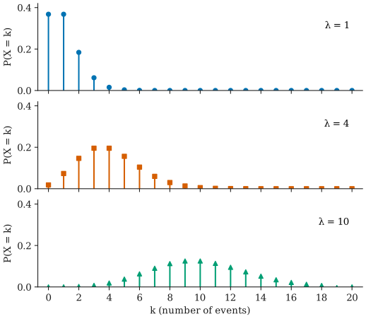
• The distribution is centred near $\lambda$. When $\lambda$ is a whole number, $\lambda - 1$ and $\lambda$ are equally likely and are the two most likely counts (for $\lambda = 1$, the counts 0 and 1 both have probability about $0.37$).
• For small $\lambda$ the distribution is strongly skewed to the right: counts cannot go below $0$, but they can occasionally be much larger than $\lambda$.
• As $\lambda$ grows, the distribution spreads out (standard deviation $\sqrt{\lambda}$) and becomes more symmetric and bell-shaped. For large $\lambda$ it is well approximated by a normal distribution with mean $\lambda$ and variance $\lambda$.

Worked example

A help desk receives on average 3 calls per hour, and calls arrive independently at a steady rate. Let $X$ be the number of calls in a given hour, so $X \sim \text{Poisson}(3)$.

Step 1: no calls.

$$P(X = 0) = e^{-3} \approx 0.0498.$$

About 5% of hours have no calls at all.

Step 2: five or more calls. It is easier to compute the complement, four or fewer, and subtract from $1$:

These add up to about $0.8153$, so

$$P(X \ge 5) \approx 1 - 0.8153 = 0.1847.$$

The desk should expect 5 or more calls in roughly 18% of hours, even though the average is only 3. This is the kind of calculation used to decide how many staff are needed.

Step 3: a longer interval. Over two hours the count is $\text{Poisson}(6)$, so the chance of two hours without a call is $e^{-6} \approx 0.0025$, about 1 in 400.

Poisson as a limit of the binomial

Let $X \sim \text{Binomial}(n, p)$ with $p = \lambda / n$, so the expected number of successes $np = \lambda$ stays fixed as $n$ grows. Then

$$P(X = k) = \binom{n}{k} \left(\frac{\lambda}{n}\right)^k \left(1 - \frac{\lambda}{n}\right)^{n-k}.$$

As $n \to \infty$ with $k$ fixed, three things happen: $\binom{n}{k} / n^k \to 1/k!$, the factor $(1 - \lambda/n)^{n}$ tends to $e^{-\lambda}$, and $(1 - \lambda/n)^{-k} \to 1$. What remains is $e^{-\lambda} \lambda^k / k!$, the Poisson PMF.

In practice, a binomial with large $n$ and small $p$ can be replaced by a Poisson with $\lambda = np$. For example, with $n = 1000$ and $p = 0.003$ (so $\lambda = 3$), the binomial gives $P(X = 0) \approx 0.04956$ and the Poisson gives $0.04979$. With only $n = 10$ and $p = 0.3$, the binomial gives $0.0282$, far from the Poisson value: the approximation needs many trials, each with a small probability.

The Poisson distribution is also closely tied to waiting times. If events follow a Poisson process with rate $\lambda$ per unit time, the time until the next event has an exponential distribution with the same rate.

When the Poisson model fails

The Poisson model assumes that events occur independently and at a constant average rate over the interval. When these assumptions fail, the most common symptom is overdispersion: the variance of the counts is larger than their mean.

• Varying rate. A help desk is busier on Monday mornings than on Sunday nights. Pooling hours with different rates gives counts that are more spread out than any single Poisson distribution.
• Clustering. Events that trigger other events, such as aftershocks following an earthquake or infections spreading between people, arrive in bursts rather than independently.
• Excess zeros. Counts of, say, fish caught per visitor include many people who never went fishing, giving more zeros than a Poisson model allows.

A quick check is to compare the sample mean and sample variance of the counts. If the variance is much larger, the Poisson model will understate uncertainty, and a model that allows extra variation (such as the negative binomial distribution) is usually more appropriate.

Common misunderstandings

“A Poisson count with mean 3 will usually be close to 3.” The standard deviation is $\sqrt{3} \approx 1.7$, and in the example values of 5 or more occur in about 18% of hours. Rare-event counts are naturally noisy.

“Any count is Poisson.” Counts with a fixed maximum, such as successes out of $n$ trials, are binomial. Counts with overdispersion or clustering are not Poisson either.

“λ must be a whole number.” It is an average, so it can be any positive number, such as $0.4$ accidents per month.

“The rate does not depend on the interval.” It does: $\lambda$ is the expected count for one particular interval length. Double the interval and you double $\lambda$.

Further reading

• Joseph K. Blitzstein and Jessica Hwang, Introduction to Probability, 2nd ed., CRC Press, 2019. Covers the Poisson distribution, its binomial limit, and Poisson processes.
• NIST/SEMATECH, e-Handbook of Statistical Methods, https://www.itl.nist.gov/div898/handbook/. A practical reference entry on the Poisson distribution, with formulas and plots.

Related articles

• Exponential Distribution — The distribution of the waiting time until the next event when events occur independently at a constant average rate.
• Normal Distribution — The bell-shaped continuous distribution described by a mean and a standard deviation.
• Variance of a Random Variable — The expected squared distance of a random variable from its mean, measuring how spread out its distribution is.