Normal Distribution

The bell-shaped continuous distribution described by a mean and a standard deviation.

Prerequisites: Probability Distributions, Expected Value, Variance of a Random Variable.

The normal distribution (also called the Gaussian distribution) is a continuous probability distribution with a symmetric, bell-shaped density. It is described by two numbers: a mean $\mu$, which says where the bell is centred, and a standard deviation $\sigma$, which says how wide it is.

It is the most important distribution in statistics. Many measurements are approximately normal, and, more importantly, averages of many independent quantities tend to be approximately normal even when the individual quantities are not. That second fact, the central limit theorem, is why the normal distribution appears throughout statistical inference.

Intuition

Think of the heights of adults of one sex in a large population, or the small errors made when repeatedly measuring the same length. Most values sit close to some typical value, values further away become steadily rarer, and deviations above and below the centre are about equally likely. A normal distribution describes exactly this pattern: a single peak at the centre, symmetric tails, and a smooth fall-off.

Two numbers are enough to describe it completely:

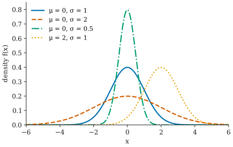
• the mean $\mu$ moves the whole curve left or right without changing its shape;
• the standard deviation $\sigma$ stretches or squeezes the curve horizontally. A larger $\sigma$ gives a wider, flatter bell; a smaller $\sigma$ gives a narrower, taller one.

Definition

A continuous random variable $X$ has a normal distribution with mean $\mu$ and variance $\sigma^2$, written $X \sim \mathcal{N}(\mu, \sigma^2)$, if its probability density function is

$$f(x) = \frac{1}{\sigma\sqrt{2\pi}} \exp\!\left( -\frac{(x-\mu)^2}{2\sigma^2} \right), \qquad -\infty < x < \infty.$$

Here:

• $x$ is a possible value of $X$, any real number;
• $\mu$ is the mean, any real number;
• $\sigma > 0$ is the standard deviation, and $\sigma^2$ is the variance;
• $\exp(u)$ means $e^u$.

Note the convention: the second parameter in $\mathcal{N}(\mu, \sigma^2)$ is the variance, not the standard deviation. Some books and software use $\sigma$ instead, so always check which one is meant.

Reading the formula

The formula has two parts.

• The exponent $-(x-\mu)^2 / (2\sigma^2)$ measures how far $x$ is from $\mu$, in units of $\sigma$. It equals $0$ at $x = \mu$, so the density is largest there, and it becomes more and more negative as $x$ moves away in either direction. Because the distance is squared, the curve is symmetric about $\mu$.
• The constant $1/(\sigma\sqrt{2\pi})$ is there only to make the total area under the curve equal to $1$, as every probability density must.

The density is not a probability

For a continuous variable, $f(x)$ is a density, not a probability. The probability that $X$ lands in an interval is the area under the density over that interval:

$$P(a \le X \le b) = \int_a^b f(x)\, dx.$$

The probability that $X$ equals any single exact value is $0$. A density value can even exceed $1$: the curve with $\sigma = 0.5$ in the figure above peaks at about $0.80$, and a curve with $\sigma = 0.1$ peaks at about $4$.

Mean and variance

If $X \sim \mathcal{N}(\mu, \sigma^2)$, then

$$\E[X] = \mu, \qquad \Var(X) = \sigma^2.$$

So the parameters are exactly the expected value and the variance of the distribution. Because the density is symmetric about $\mu$, the mean, median, and mode are all equal to $\mu$.

The standard normal distribution

The normal distribution with $\mu = 0$ and $\sigma = 1$ is called the standard normal distribution. A standard normal variable is usually written $Z$, its density $\varphi(z)$ and its cumulative distribution function (CDF) $\Phi(z) = P(Z \le z)$.

Any normal variable can be converted to a standard normal one by subtracting its mean and dividing by its standard deviation:

$$Z = \frac{X - \mu}{\sigma} \sim \mathcal{N}(0, 1).$$

The value $z = (x - \mu)/\sigma$ is called a z-score. It says how many standard deviations $x$ lies above (positive) or below (negative) the mean. This standardization is why one table of $\Phi$, or one software function, is enough to compute probabilities for every normal distribution:

$$P(X \le x) = \Phi\!\left(\frac{x - \mu}{\sigma}\right).$$

There is no formula for $\Phi$ in terms of elementary functions; it is computed numerically. In Python, for example, scipy.stats.norm.cdf(z) returns $\Phi(z)$.

The 68–95–99.7 rule

For every normal distribution, the probability of landing within a fixed number of standard deviations of the mean is the same:

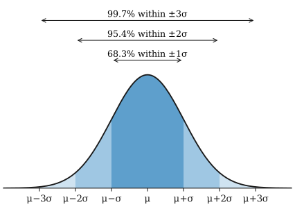
This gives a quick sense of scale. A value two standard deviations from the mean is unusual (it happens about 1 time in 22), and a value more than three standard deviations away is rare (about 1 time in 370). The often-quoted “95% within 2 standard deviations” is a rounding: the exact multiplier for 95% is $1.96$.

Worked example

Scores on a standardized test are approximately normal with mean $\mu = 500$ and standard deviation $\sigma = 100$. What fraction of test-takers score below 650?

Step 1: standardize. The z-score of 650 is

$$z = \frac{650 - 500}{100} = 1.5.$$

So 650 is one and a half standard deviations above the mean.

Step 2: look up the standard normal CDF. $\Phi(1.5) \approx 0.9332$. About 93.3% of test-takers score below 650, and about 6.7% score above it.

A second question: what fraction score between 400 and 700? The z-scores are $-1$ and $2$, so

$$P(400 \le X \le 700) = \Phi(2) - \Phi(-1) \approx 0.9772 - 0.1587 = 0.8186.$$

About 82% of test-takers score in this range. As a check, the answer lies between the 68% for $\pm 1\sigma$ and the 95% for $\pm 2\sigma$, which makes sense for an interval running from $-1\sigma$ to $+2\sigma$.

Where the normal distribution appears

• Measurement error. Small errors made up of many tiny independent disturbances tend to be approximately normal.
• Averages and sums. By the central limit theorem, the mean of a large sample is approximately normal, whatever the shape of the population. This is the basis of many confidence intervals and hypothesis tests.
• Approximations to other distributions. A binomial distribution with many trials, or a Poisson distribution with a large mean, is close to normal.
• Modelling assumptions. Linear regression often assumes normally distributed errors when deriving tests and intervals.

Common misunderstandings

“Most data are normal.” Many are not. Incomes, waiting times, and counts of rare events are typically skewed; some data have heavier tails than a normal distribution allows. The normal distribution is a useful model, not a law of nature. Look at a histogram before assuming it.

“The normal distribution can produce any value, so it cannot model heights.” Strictly, a normal variable can take negative values, which a height cannot. But if the mean is many standard deviations above zero, the probability of a negative value is so small that the model is still excellent in practice.

“The density at a point is the probability of that point.” It is not; see above. For a continuous variable, only areas are probabilities.

“Within 2σ means exactly 95%.” It means about 95.4%. The 95% interval is $\mu \pm 1.96\sigma$.

Further reading

• Joseph K. Blitzstein and Jessica Hwang, Introduction to Probability, 2nd ed., CRC Press, 2019. The chapter on continuous random variables covers the normal distribution and standardization.
• David M. Diez, Mine Çetinkaya-Rundel, and Christopher D. Barr, OpenIntro Statistics, 4th ed., 2019. Free online; includes many worked normal-probability examples.

Related articles

• Central Limit Theorem — The mean of many independent observations is approximately normally distributed, whatever the shape of the population.
• Sampling Distributions — The distribution of a statistic, such as the sample mean, over all the samples that could have been drawn.
• Confidence Intervals — A range of plausible values for a parameter, produced by a procedure that captures the true value in a stated fraction of repeated samples.
• Bernoulli and Binomial Distributions — The distributions of a single yes/no trial and of the number of successes in a fixed number of independent trials.