Simple Linear Regression

Fitting a straight line to predict one variable from another by minimizing the sum of squared residuals.

Prerequisites: Correlation, Variance and Standard Deviation.

Simple linear regression fits a straight line through a scatter plot so that one variable, $y$, can be described or predicted from another, $x$. The line is chosen by least squares: it makes the vertical distances from the points to the line, squared and added up, as small as possible.

It is the simplest statistical model of how one quantity changes with another, and the starting point for nearly all of regression modelling. The fitted slope answers a concrete question, such as “how many extra exam points go with one extra hour of study, on average?”, and the same ideas (residuals, least squares, $R^2$) carry over to models with many predictors.

Intuition

Plot exam scores $y$ against hours studied $x$ for a class, and the points rise roughly along a line, with scatter around it. Many lines could be drawn through the cloud. To pick one, we measure how badly each candidate line misses: for each student, the residual is the vertical gap between the observed score and the score the line predicts. Least squares picks the line whose squared residuals have the smallest total.

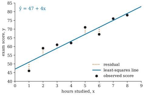
Why vertical distances? Because the goal is to predict $y$ from $x$: the residual is the prediction error in the units of $y$. Why squares? Squaring makes every error count as positive, penalizes large misses heavily, and, as shown below, leads to simple closed-form answers.

The model

We observe $n$ pairs $(x_1, y_1), \dots, (x_n, y_n)$. Simple linear regression assumes

$$y_i = \beta_0 + \beta_1 x_i + \varepsilon_i, \qquad i = 1, \dots, n,$$

where:

• $\beta_0$ is the intercept: the mean of $y$ when $x = 0$;
• $\beta_1$ is the slope: the change in the mean of $y$ for a one-unit increase in $x$;
• $\varepsilon_i$ is the error for observation $i$: everything about $y_i$ that the line does not capture, such as other influences and measurement noise.

The parameters $\beta_0$ and $\beta_1$ are unknown population quantities. We estimate them from the data by $\hat{\beta}_0$ and $\hat{\beta}_1$ (the hats mark estimates), giving the fitted line

$$\hat{y} = \hat{\beta}_0 + \hat{\beta}_1 x.$$

Assumptions

The usual assumptions, roughly in order of importance:

1. Linearity. The mean of $y$ really does change linearly with $x$: $\E[\varepsilon_i] = 0$ for every $x_i$. If the true relationship is curved, the line is a poor summary no matter how it is fitted.
2. Independent errors. The errors for different observations are independent. This fails, for example, for repeated measurements on the same person or for data collected over time.
3. Constant variance. The errors have the same variance $\sigma^2$ at every value of $x$. If the scatter fans out as $x$ grows, this fails.
4. Normal errors. The errors follow a normal distribution, $\varepsilon_i \sim \mathcal{N}(0, \sigma^2)$.

The least-squares line itself can be computed without any of these assumptions; they matter for interpreting it and for inference. Normality is needed only for exact confidence intervals and hypothesis tests in small samples. With larger samples, those procedures remain approximately valid without it, by the central limit theorem. The other three assumptions cannot be rescued by a larger sample.

Least squares

For a candidate intercept $b_0$ and slope $b_1$, the residual of point $i$ is $y_i - (b_0 + b_1 x_i)$. The sum of squared residuals is

$$\text{SSE}(b_0, b_1) = \sum_{i=1}^n \big(y_i - b_0 - b_1 x_i\big)^2.$$

The least-squares estimates $\hat{\beta}_0, \hat{\beta}_1$ are the values of $b_0, b_1$ that minimize it. Writing

$$S_{xx} = \sum_{i=1}^n (x_i - \bar{x})^2, \qquad S_{xy} = \sum_{i=1}^n (x_i - \bar{x})(y_i - \bar{y}),$$

the solution is

$$\hat{\beta}_1 = \frac{S_{xy}}{S_{xx}}, \qquad \hat{\beta}_0 = \bar{y} - \hat{\beta}_1 \bar{x}.$$

This requires $S_{xx} > 0$, that is, the $x$ values are not all equal.

Where the formulas come from

SSE is a smooth bowl-shaped function of $b_0$ and $b_1$, so its minimum is where both partial derivatives are zero. Writing $e_i = y_i - b_0 - b_1 x_i$, the two conditions are

$$\sum_{i=1}^n e_i = 0, \qquad \sum_{i=1}^n x_i e_i = 0.$$

The first condition says the residuals sum to zero. Dividing it by $n$ gives $\bar{y} - b_0 - b_1\bar{x} = 0$, so $b_0 = \bar{y} - b_1 \bar{x}$: the least-squares line always passes through the point of means $(\bar{x}, \bar{y})$.

Substituting this into $e_i$ gives $e_i = (y_i - \bar{y}) - b_1(x_i - \bar{x})$. Because $\sum e_i = 0$, the second condition can be rewritten as $\sum (x_i - \bar{x}) e_i = 0$, which becomes

$$\sum_{i=1}^n (x_i - \bar{x})(y_i - \bar{y}) - b_1 \sum_{i=1}^n (x_i - \bar{x})^2 = 0,$$

that is, $S_{xy} - b_1 S_{xx} = 0$, so $b_1 = S_{xy}/S_{xx}$.

The slope in terms of correlation

Dividing the top and bottom of $S_{xy}/S_{xx}$ by $n - 1$ turns them into the sample covariance $s_{xy}$ and the sample variance $s_x^2$. Since the sample correlation is $r = s_{xy}/(s_x s_y)$,

$$\hat{\beta}_1 = \frac{s_{xy}}{s_x^2} = r\,\frac{s_y}{s_x}.$$

The slope is the correlation, rescaled from “standard deviations of $y$ per standard deviation of $x$” into the actual units of $y$ per unit of $x$.

Interpreting the fit

• Slope. $\hat{\beta}_1$ is the estimated change in the average of $y$ associated with a one-unit increase in $x$. It describes the trend across the population, not what will happen to any individual.
• Intercept. $\hat{\beta}_0$ is the predicted $y$ at $x = 0$. It is meaningful only if $x = 0$ is a sensible value inside or near the range of the data; otherwise it is just the number that positions the line.
• Residuals. The residuals $e_i = y_i - \hat{y}_i$ are what the line leaves unexplained. Their typical size is summarized by the residual standard deviation $s_e = \sqrt{\text{SSE}/(n - 2)}$, which estimates the error standard deviation $\sigma$. The divisor is $n - 2$ because two parameters were estimated from the data.

R² and the fraction of variance explained

The total variation of $y$ around its mean, $\text{SST} = \sum (y_i - \bar{y})^2$, splits into a part explained by the line and a part left in the residuals:

$$\underbrace{\sum_{i=1}^n (y_i - \bar{y})^2}_{\text{SST}} = \underbrace{\sum_{i=1}^n (\hat{y}_i - \bar{y})^2}_{\text{explained}} + \underbrace{\sum_{i=1}^n (y_i - \hat{y}_i)^2}_{\text{SSE}}.$$

The coefficient of determination is the explained fraction:

$$R^2 = 1 - \frac{\text{SSE}}{\text{SST}}.$$

It lies between $0$ (the line does no better than predicting $\bar{y}$ for everyone) and $1$ (every point lies on the line). In simple linear regression, $R^2 = r^2$, the square of the sample correlation between $x$ and $y$.

Worked example

Eight students record how many hours $x$ they studied for an exam and their score $y$ out of 100.

Step 1: means. $\bar{x} = 36/8 = 4.5$ hours and $\bar{y} = 520/8 = 65$ points.

Step 2: slope. From the column sums, $S_{xx} = 42$ and $S_{xy} = 168$, so

$$\hat{\beta}_1 = \frac{168}{42} = 4 \text{ points per hour}.$$

Step 3: intercept.

$$\hat{\beta}_0 = \bar{y} - \hat{\beta}_1 \bar{x} = 65 - 4 \times 4.5 = 47 \text{ points}.$$

The fitted line is $\hat{y} = 47 + 4x$. Each additional hour of study is associated with 4 more points on average. The intercept, 47, is the predicted score for a student who did not study at all; that is slightly outside the data (the minimum was 1 hour), so treat it with some caution.

Step 4: residuals. The fitted values at $x = 1, \dots, 8$ are $51, 55, 59, 63, 67, 71, 75, 79$, so the residuals are

$$-5,\ 4,\ 2,\ -1,\ 4,\ -4,\ 1,\ -1.$$

They sum to zero, as least squares guarantees. Their squares sum to $\text{SSE} = 80$, and the residual standard deviation is $s_e = \sqrt{80/6} \approx 3.65$ points: a typical student’s score lies within a few points of the line.

Step 5: R². The squared deviations $(y_i - \bar{y})^2$ sum to $\text{SST} = 752$. So

$$R^2 = 1 - \frac{80}{752} \approx 0.894.$$

About 89% of the variation in scores among these students is accounted for by the linear relationship with hours studied. As a check, $r = 168/\sqrt{42 \times 752} \approx 0.945$, and $r^2 \approx 0.894$. Also $s_x = \sqrt{42/7} \approx 2.45$ and $s_y = \sqrt{752/7} \approx 10.36$, and $r\, s_y/s_x \approx 0.945 \times 10.36 / 2.45 \approx 4$, matching the slope.

Step 6: predict. For a student who studies 5.5 hours, the line predicts $47 + 4 \times 5.5 = 69$ points.

Checking the assumptions with residual plots

The scatter plot with the fitted line is the first check. The second is a residual plot: residuals $e_i$ on the vertical axis against $x_i$ (or against the fitted values $\hat{y}_i$). If the assumptions hold, the residuals form a shapeless horizontal band around zero. Typical warning signs:

• A curve (residuals positive at both ends and negative in the middle, or the reverse): the relationship is not linear.
• A funnel (residuals spreading out as $x$ grows): the variance is not constant.
• One or two isolated points far from zero: outliers, which can pull the line towards themselves, much as one point can distort a correlation.
• Trends in the order the data were collected: the errors may not be independent.

A histogram or normal quantile plot of the residuals can check normality, but with small samples such checks have little power, and with large samples normality matters less.

Regression to the mean

Dividing both sides of the fitted line by the standard deviations shows that, in z-score units, the predicted $y$ is

$$\frac{\hat{y} - \bar{y}}{s_y} = r \, \frac{x - \bar{x}}{s_x}.$$

Unless the points lie exactly on a line, $|r| < 1$, so the prediction is always fewer standard deviations from the mean than $x$ is. In the example, a student who studies one standard deviation above average (about 6.95 hours) is predicted to score $0.945$ standard deviations above average, not a full one.

This is regression to the mean, and it is where the word “regression” comes from: Francis Galton observed in the 19th century that unusually tall parents tend to have children who are tall, but less extremely so. It is a statistical effect, not a causal force. It also explains many apparent “treatment effects”: a group selected because it scored unusually badly will, on average, score closer to the mean next time even if nothing is done.

Limitations

Extrapolation. The line describes the data in the range where it was observed. Outside that range there is no evidence that the relationship stays linear. Our line predicts $47 + 4 \times 20 = 127$ points for a student who studies 20 hours, which is impossible on a test out of 100. Predictions far from the observed $x$ values deserve little trust.

Causation. A regression of $y$ on $x$ describes association, just like correlation. In the example, students who study more may also attend more classes or have more prior knowledge, and these confounders could explain part of the slope. Interpreting $\hat{\beta}_1$ as “the effect of one more hour of study” needs a randomized experiment or a careful argument that confounding is absent.

Direction matters. Regressing $y$ on $x$ and regressing $x$ on $y$ give different lines (unless $r = \pm 1$), because one minimizes vertical distances and the other horizontal ones. Choose the variable you want to predict as $y$.

Common misunderstandings

“A high R² means the model is correct.” A curved relationship can still give a high $R^2$ for a straight line, and a line with high $R^2$ can still violate the assumptions. Look at the residual plot.

“A low R² means x has no effect.” A small $R^2$ means $x$ explains little of the variation in $y$, but the slope can still be real and important, especially when $y$ has many other influences.

“The slope tells us what happens when we change x.” Only under causal assumptions. Without them it describes how the average of $y$ differs between groups with different $x$.

“Normality of the data is required to fit a regression.” Least squares can be computed for any data. Normality concerns the errors, not $x$ or $y$ themselves, and it matters only for exact small-sample inference.

Further reading

• David Freedman, Robert Pisani, and Roger Purves, Statistics, 4th ed., W. W. Norton, 2007. Explains regression, the regression effect, and their misuses with unusual clarity.
• David M. Diez, Mine Çetinkaya-Rundel, and Christopher D. Barr, OpenIntro Statistics, 4th ed., 2019. Free online; covers least squares, residual plots, and inference for the slope.
• NIST/SEMATECH, e-Handbook of Statistical Methods, https://www.itl.nist.gov/div898/handbook/. A practical reference on fitting and checking regression models.

Related articles

• Covariance — A measure of whether two variables tend to be above and below their means at the same time.
• Normal Distribution — The bell-shaped continuous distribution described by a mean and a standard deviation.
• Hypothesis Testing — A procedure for deciding whether data are inconsistent enough with a default claim about a population to reject that claim.
• Confidence Intervals — A range of plausible values for a parameter, produced by a procedure that captures the true value in a stated fraction of repeated samples.