Covariance

A measure of whether two variables tend to be above and below their means at the same time.

Prerequisites: Expected Value, Variance of a Random Variable, Variance and Standard Deviation.

Covariance measures whether two variables tend to move together. It is positive when large values of one variable tend to go with large values of the other, negative when large values of one tend to go with small values of the other, and near zero when there is no such linear tendency.

Covariance is rarely reported on its own, because its size depends on the units of measurement. But it is the building block of correlation and linear regression, and it appears whenever we add random quantities together, so it is worth understanding well.

Intuition

Suppose we record, for many people, the number of hours they practise a skill and their score on a test of it. For each person, ask two questions: is their practice time above or below the average, and is their score above or below the average?

• If people who practise more than average also tend to score more than average (and those who practise less tend to score less), the two deviations usually have the same sign.
• If the opposite happens, the two deviations usually have opposite signs.

Covariance turns this into a number. For each observation it multiplies the deviation of $x$ from its mean by the deviation of $y$ from its mean. The product is positive when both deviations have the same sign and negative when they differ. Averaging the products tells us which kind of observation dominates.

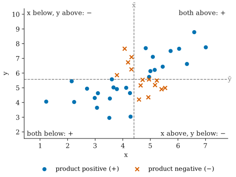
The dashed lines in the figure split the plane into four quadrants. Points in the upper-right and lower-left quadrants contribute positive products; points in the other two contribute negative products. A point far from both means contributes a large product, and a point near either dashed line contributes almost nothing. The covariance is, roughly, the average of all these signed contributions.

Definition

Population covariance

Let $X$ and $Y$ be two random variables defined on the same population, with means $\mu_X = \E[X]$ and $\mu_Y = \E[Y]$. Their covariance is the expected value of the product of their deviations from their means:

$$\Cov(X, Y) = \E\big[(X - \mu_X)(Y - \mu_Y)\big].$$

Expanding the product and using linearity of expectation gives an equivalent formula that is often easier to compute:

$$\Cov(X, Y) = \E[XY] - \E[X]\,\E[Y].$$

To see why, multiply out: $(X - \mu_X)(Y - \mu_Y) = XY - \mu_Y X - \mu_X Y + \mu_X \mu_Y$. Taking expectations, the middle two terms each become $\mu_X \mu_Y$, so the right-hand side is $\E[XY] - \mu_X\mu_Y - \mu_X\mu_Y + \mu_X\mu_Y = \E[XY] - \mu_X\mu_Y$.

For discrete variables with joint probability mass function $p(x, y) = P(X = x, Y = y)$, the expectation is a sum, $\Cov(X, Y) = \sum_x \sum_y (x - \mu_X)(y - \mu_Y)\, p(x, y)$. For continuous variables it is the corresponding integral against the joint density.

Sample covariance

From a sample of $n$ pairs $(x_1, y_1), \dots, (x_n, y_n)$ with sample means $\bar{x}$ and $\bar{y}$, the sample covariance is

$$s_{xy} = \frac{1}{n - 1} \sum_{i=1}^n (x_i - \bar{x})(y_i - \bar{y}).$$

It estimates $\Cov(X, Y)$. The divisor $n - 1$ rather than $n$ plays the same role as in the sample variance: it corrects for measuring deviations from the sample means instead of the unknown population means, and makes $s_{xy}$ an unbiased estimator. With $n - 1$, the sample covariance of $x$ with itself is exactly the sample variance $s_x^2$.

Reading the sign

• $\Cov(X, Y) > 0$: above-average values of $X$ tend to occur with above-average values of $Y$.
• $\Cov(X, Y) < 0$: above-average values of $X$ tend to occur with below-average values of $Y$.
• $\Cov(X, Y) = 0$: the variables are uncorrelated. There is no linear tendency, but, as explained below, there may still be a strong relationship of another kind.

Worked example

Five basketball players report the hours $x$ they practised free throws last week, and then each takes 10 free throws; $y$ is the number made.

Step 1: compute the means. $\bar{x} = (1+2+3+4+5)/5 = 3$ hours and $\bar{y} = (2+4+5+4+5)/5 = 4$ throws.

Step 2: tabulate deviations and their products.

The deviations in each column sum to zero, as they always must. Player 1 (below average on both) and player 5 (above average on both) contribute positive products; nobody contributes a negative one.

Step 3: divide by $n - 1$.

$$s_{xy} = \frac{6}{5 - 1} = 1.5 \text{ hour-throws}.$$

The covariance is positive: in this small sample, more practice goes with more successful throws.

Step 4: notice the units. The unit is “hours × throws”, which has no natural meaning. Worse, if we had recorded practice in minutes, every $x_i - \bar{x}$ would be 60 times larger, and the covariance would be $60 \times 1.5 = 90$, even though the data describe exactly the same relationship. The number 1.5 cannot tell us whether the relationship is strong or weak.

The scale problem and correlation

The worked example shows the main weakness of covariance: its magnitude depends on the units of both variables. In general, for constants $a$ and $c$,

$$\Cov(aX, cY) = ac\,\Cov(X, Y).$$

So covariance tells us the direction of a linear relationship but not, by itself, its strength. Dividing by the two standard deviations removes the units and gives the correlation coefficient, which always lies between $-1$ and $1$. For the free-throw data, the sample standard deviations are $s_x = \sqrt{10/4} \approx 1.58$ and $s_y = \sqrt{6/4} \approx 1.22$, and the correlation is $1.5 / (1.58 \times 1.22) \approx 0.77$, whichever units we use.

Properties

The following hold for any random variables with finite variances, and for any constants $a, b, c, d$.

Covariance with itself is variance.

$$\Cov(X, X) = \E\big[(X - \mu_X)^2\big] = \Var(X).$$

Symmetry. $\Cov(X, Y) = \Cov(Y, X)$.

Shifts do not matter; scaling multiplies. Adding a constant moves a variable and its mean by the same amount, so deviations are unchanged:

$$\Cov(aX + b, \, cY + d) = ac\,\Cov(X, Y).$$

Additivity. $\Cov(X + Y, Z) = \Cov(X, Z) + \Cov(Y, Z)$. Together with the previous rule, this says covariance is linear in each argument (it is bilinear).

Variance of a sum. Applying these rules to $\Var(X + Y) = \Cov(X + Y, X + Y)$ gives

$$\Var(X + Y) = \Var(X) + \Var(Y) + 2\Cov(X, Y).$$

When $X$ and $Y$ move together, their sum varies more than the two variances alone would suggest; when they move in opposite directions, they partly cancel and the sum varies less. Only when $\Cov(X, Y) = 0$ do the variances simply add. The same identity holds for sample quantities: for the free-throw data, the values $x_i + y_i$ are $3, 6, 8, 8, 10$, whose sample variance is $28/4 = 7$, which equals $s_x^2 + s_y^2 + 2s_{xy} = 2.5 + 1.5 + 3$.

Independence and zero covariance

If $X$ and $Y$ are independent, then $\E[XY] = \E[X]\,\E[Y]$, and so $\Cov(X, Y) = 0$. Independent variables are always uncorrelated.

The converse is false: zero covariance does not imply independence. Covariance only detects linear tendencies, and a relationship can be perfectly strong yet not linear.

A standard example: let $X$ take the values $-1$, $0$, $1$, each with probability $1/3$, and let $Y = X^2$. Then $Y$ is completely determined by $X$. Yet

$$\E[X] = 0, \qquad \E[XY] = \E[X^3] = \tfrac{1}{3}(-1 + 0 + 1) = 0,$$

so $\Cov(X, Y) = 0 - 0 \cdot \E[Y] = 0$. The variables are not independent: $P(Y = 1) = 2/3$, but once we know $X = 1$, we know $Y = 1$ for certain. The covariance is zero because the positive products from $X = 1$ exactly cancel the negative products from $X = -1$. The same thing happens with $Y = X^2$ for any $X$ whose distribution is symmetric about $0$ (and has a finite third moment).

Common misunderstandings

“A large covariance means a strong relationship.” Not necessarily. Covariance grows with the spread of each variable and depends on the units. Changing hours to minutes multiplied the covariance by 60 without changing the data. Use correlation to judge strength.

“Zero covariance means the variables are unrelated.” It means there is no linear relationship. $Y = X^2$ with $X$ symmetric about zero has zero covariance with $X$ even though $Y$ is a function of $X$. Always look at a scatter plot.

“Positive covariance means one variable causes the other.” Covariance describes how variables vary together in the data; it says nothing about why. A third variable can drive both.

“Variances of a sum always add.” Only when the covariance is zero, for example when the variables are independent. Otherwise the $2\Cov(X, Y)$ term matters, and it can be large.

Further reading

• Joseph K. Blitzstein and Jessica Hwang, Introduction to Probability, 2nd ed., CRC Press, 2019. Covers covariance, correlation, and joint distributions with many examples.
• Larry Wasserman, All of Statistics: A Concise Course in Statistical Inference, Springer, 2004. A compact treatment of covariance and its properties.

Related articles

• Correlation — A unit-free number between −1 and 1 that measures the strength and direction of a linear relationship between two variables.
• Statistical Independence — Two events are independent when knowing that one happened does not change the probability of the other.
• Simple Linear Regression — Fitting a straight line to predict one variable from another by minimizing the sum of squared residuals.