Variance and Standard Deviation

Measures of how far data values typically lie from their mean, including why the sample variance divides by n − 1.

Prerequisites: Mean, Median, and Mode.

The standard deviation measures how spread out a set of values is around its mean: roughly, how far a typical value lies from the average. The variance is the square of the standard deviation. A small standard deviation means the values cluster tightly around the mean; a large one means they are widely scattered.

Knowing the centre of a dataset is only half the picture. Two classes can have the same average exam score while one has nearly everyone near the average and the other has a mix of very high and very low scores. The standard deviation is the most widely used number for describing that difference, and it appears throughout statistics, from the normal distribution to confidence intervals.

Intuition

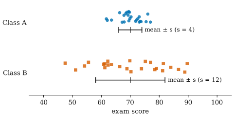
Both classes in the figure have a mean of 70. In class A almost everyone scored within a few points of 70; in class B scores range from below 50 to almost 90. The standard deviation puts a number on this: 4 points for class A, 12 for class B.

The natural way to measure spread is to look at each value’s deviation from the mean, $x_i - \bar{x}$, and ask how large these deviations typically are. Two problems arise:

1. Deviations cancel. Positive and negative deviations always add up to exactly zero, because the mean is the balance point of the data. So the average deviation is always 0 and says nothing.
2. We need a size, not a sign. We have to remove the signs before averaging.

Squaring each deviation solves both problems: squares are never negative, and larger deviations count for more. Averaging the squared deviations gives the variance. Because squaring also squares the units (points become “points squared”), we take the square root at the end to get back to the original units. That is the standard deviation.

Why square rather than take absolute values? Both are legitimate; the mean absolute deviation is a perfectly good measure of spread. Squares are preferred because they behave much better mathematically. For example, the variance of a sum of independent quantities is the sum of their variances, a fact with no equally simple counterpart for absolute deviations, and the mean is exactly the value that minimizes the sum of squared deviations (see mean, median, and mode).

Definitions

Population variance and standard deviation

If the data are an entire population of $N$ values $x_1, \dots, x_N$ with mean $\mu$, the population variance is the average squared deviation:

$$\sigma^2 = \frac{1}{N} \sum_{i=1}^N (x_i - \mu)^2 ,$$

and the population standard deviation is $\sigma = \sqrt{\sigma^2}$. Here $\sigma$ is the Greek letter sigma. The variance of a probability distribution is defined in the same spirit, as an expected squared deviation; see variance of a random variable.

Sample variance and standard deviation

Usually the data are a sample of $n$ values $x_1, \dots, x_n$ from a larger population, and we do not know $\mu$. We measure deviations from the sample mean $\bar{x}$ instead, and divide by $n - 1$ rather than $n$:

$$s^2 = \frac{1}{n-1} \sum_{i=1}^n (x_i - \bar{x})^2 .$$

This is the sample variance, and $s = \sqrt{s^2}$ is the sample standard deviation. It requires $n \ge 2$. Most software computes $s$ by default when asked for a “standard deviation”, but not all: in Python, NumPy’s np.std(x) divides by $n$ unless you pass ddof=1, while pandas and R divide by $n - 1$.

Why divide by n − 1?

Dividing by $n - 1$ is called Bessel’s correction. The reason is that deviations from the sample mean are, on average, a little too small.

The sample mean $\bar{x}$ is computed from the same data, so it sits right in the middle of them. In fact, $\bar{x}$ is the value $c$ that makes $\sum_i (x_i - c)^2$ as small as possible. Unless $\bar{x}$ happens to equal $\mu$ exactly, the sum of squared deviations from $\bar{x}$ is therefore smaller than the sum of squared deviations from the true mean $\mu$. Dividing by $n$ would systematically underestimate the population variance.

How much too small? If $x_1, \dots, x_n$ are independent draws from a population with variance $\sigma^2$, then on average

$$\E\!\left[ \sum_{i=1}^n (x_i - \bar{x})^2 \right] = (n - 1)\,\sigma^2 .$$

So dividing by $n - 1$ gives an estimate that is right on average, $\E[s^2] = \sigma^2$, whereas dividing by $n$ gives an average of $\frac{n-1}{n}\sigma^2$. With $n = 5$ that is only 80% of the true variance. In the language of point estimation, $s^2$ is an unbiased estimator of $\sigma^2$.

A second way to see it is through degrees of freedom. The $n$ deviations $x_i - \bar{x}$ always add up to zero, so once you know $n - 1$ of them, the last one is determined. Only $n - 1$ of them carry independent information about spread. The extreme case makes this vivid: with a single observation ($n = 1$), the only deviation is $x_1 - \bar{x} = 0$. One value tells you nothing about spread, and the formula, which would divide by zero, refuses to pretend otherwise.

Two remarks keep this in proportion. First, for large $n$ the difference between dividing by $n$ and by $n - 1$ is negligible. Second, although $s^2$ is unbiased for $\sigma^2$, its square root $s$ is slightly biased (on average a little too small) as an estimate of $\sigma$. It is still the standard choice.

Worked example

Five students score 6, 8, 9, 11, and 16 points on a quiz. We treat them as a sample and compute $s$ by hand.

Step 1: the mean. $\bar{x} = (6 + 8 + 9 + 11 + 16)/5 = 50/5 = 10$ points.

Step 2: deviations and their squares.

As expected, the deviations add up to 0. The score of 16, far from the mean, contributes 36 of the 58: squaring makes large deviations dominate.

Step 3: the sample variance. Divide the sum of squares by $n - 1 = 4$:

$$s^2 = \frac{58}{4} = 14.5 \text{ points}^2 .$$

Step 4: the sample standard deviation.

$$s = \sqrt{14.5} \approx 3.81 \text{ points}.$$

A typical score lies roughly 4 points from the mean of 10, which matches a glance at the data.

Step 5: compare with dividing by n. If these five students were the entire population of interest, we would divide by $N = 5$: $\sigma^2 = 58/5 = 11.6$ and $\sigma \approx 3.41$ points. The two answers differ noticeably here because $n$ is small.

Interpreting the standard deviation

The standard deviation is in the same units as the data, so it can be read directly: “scores averaged 70 with a standard deviation of 4 points”.

For data that are roughly bell-shaped, the 68–95–99.7 rule gives a useful scale: about 68% of values within one standard deviation of the mean, and about 95% within two. For any dataset, whatever its shape, at least 75% of the values lie within two standard deviations of the mean (a consequence of Chebyshev’s inequality), but the bell-curve percentages may not apply.

The number of standard deviations a value lies from the mean, $(x - \bar{x})/s$, is its z-score. It puts measurements on different scales onto a common one: a z-score of 2 means “two standard deviations above average”, whether the original units were points, centimetres, or seconds.

Two simple rules describe how the standard deviation reacts to changes in the data:

• Adding a constant to every value shifts the mean but leaves the standard deviation unchanged. Spread does not depend on location.
• Multiplying every value by a constant $a$ multiplies the standard deviation by $|a|$ and the variance by $a^2$. Converting metres to centimetres multiplies $s$ by 100.

Common misunderstandings

“The standard deviation is the average distance from the mean.” Not exactly. It is the square root of the average squared distance, which gives extra weight to large deviations; it is usually somewhat larger than the mean absolute deviation. “A typical distance” is a fair informal description.

“Variance and standard deviation are interchangeable.” They carry the same information, but only the standard deviation is in the original units. A variance of 14.5 points² is hard to interpret directly; a standard deviation of 3.8 points is not.

“A small standard deviation means the data are accurate.” It means they are consistent with each other. A scale that always reads 2 kg too heavy has a small standard deviation and a large bias.

“The standard deviation of a sample tells you how precise its mean is.” It describes the spread of individual values. The precision of the sample mean is described by the standard error, which shrinks as the sample grows; see sampling distributions.

“The standard deviation is robust.” Because deviations are squared, a single extreme value can inflate it a lot. For skewed data or data with outliers, the interquartile range is often a better summary of spread.

Further reading

• David Freedman, Robert Pisani, and Roger Purves, Statistics, 4th ed., W. W. Norton, 2007. Explains the standard deviation as a typical size of deviations, with many examples.
• Larry Wasserman, All of Statistics: A Concise Course in Statistical Inference, Springer, 2004. A concise, more mathematical treatment, including the unbiasedness of the sample variance.

Related articles

• Variance of a Random Variable — The expected squared distance of a random variable from its mean, measuring how spread out its distribution is.
• Quantiles, Percentiles, and Outliers — Values that cut ordered data into given proportions, the interquartile range, and how to find and handle unusual observations.
• Normal Distribution — The bell-shaped continuous distribution described by a mean and a standard deviation.
• Point Estimation — Using a single number computed from a sample to estimate an unknown population parameter, and judging how good that rule is.