Mean, Median, and Mode

Three ways to describe the typical value of a dataset, how they differ, and when to use which.

The mean, median, and mode are three ways to summarize a dataset by a single “typical” value. The mean is the ordinary average; the median is the middle value once the data are sorted; the mode is the most common value. They are called measures of centre (or of central tendency).

They often give similar answers, but not always, and the differences are informative. When they disagree, the choice between them can change the story a set of numbers seems to tell.

Intuition

Each measure answers a slightly different question.

The mean asks: if the total were shared out equally, how much would each observation get? It is the balance point of the data: imagine the values as equal weights on a ruler; the ruler balances at the mean.
The median asks: which value splits the data into two equal halves? Half the observations are at or below it, half at or above.
The mode asks: which value occurs most often?

The balance-point picture explains the most important difference. Moving one weight far out along the ruler shifts the balance point, however many other weights there are. The median only cares about which values are above and which below the middle, not how far away they are.

Definitions

Let $x_1, \dots, x_n$ be $n$ observed values.

The mean (or arithmetic mean, or average) is

\bar{x} = \frac{1}{n} \sum_{i=1}^n x_i = \frac{x_1 + x_2 + \dots + x_n}{n}.

For a whole population the mean is written $\mu$ ; the mean of a probability distribution is its expected value.

The median is found by sorting the values from smallest to largest:

if $n$ is odd, the median is the middle value, in position $(n+1)/2$ ;
if $n$ is even, it is the average of the two middle values, in positions $n/2$ and $n/2 + 1$ .

The mode is the value that occurs most often. A dataset can have two modes (bimodal), several, or effectively none if every value occurs once. For continuous measurements, where exact repeats are rare, “the mode” usually means the location of the highest peak of a histogram or density curve.

Which measures make sense depends on the type of data. The mode works for any variable, including categories such as “most common blood type”. The median needs ordered values. The mean needs numbers whose differences are meaningful.

Worked example

A small firm has seven employees with annual salaries, in thousands of euros:

32,\; 35,\; 35,\; 38,\; 41,\; 44,\; 180.

The 180 is the owner’s salary.

Step 1: mean. The total is $32 + 35 + 35 + 38 + 41 + 44 + 180 = 405$ , so

\bar{x} = \frac{405}{7} \approx 57.9 \text{ thousand euros}.

Step 2: median. The values are already sorted and $n = 7$ is odd, so the median is the 4th value: 38 thousand euros.

Step 3: mode. The value 35 occurs twice and every other value once, so the mode is 35 thousand euros.

Step 4: compare. Six of the seven employees earn less than the mean. The mean is not “typical” of anyone here; the single large salary has dragged it upward. The median, 38, is a much better description of what a typical employee earns.

Step 5: remove the outlier. Without the owner, the six remaining salaries have mean $225/6 = 37.5$ and median $(35 + 38)/2 = 36.5$ . Removing one value moved the mean by more than 20 thousand euros, but the median by only 1.5.

Robustness

A summary is robust if a few extreme or erroneous values cannot change it much. The median is robust: you could raise the three largest salaries above by any amounts at all, and the median would stay at 38. The mean is not: changing a single value by an amount $d$ changes the mean by $d/n$ , with no limit.

Robustness is not automatically good. The mean uses the size of every observation, which is exactly what you want when totals matter. If a city wants to know the total water use of its households, the mean (times the number of households) is the relevant figure, and the large users are a real part of it.

A useful way to see the difference: the mean is the number $c$ that makes the sum of squared distances $\sum_i (x_i - c)^2$ as small as possible, while the median makes the sum of absolute distances $\sum_i |x_i - c|$ as small as possible. Squaring gives large distances much more weight, which is why the mean chases outliers. The first fact is the starting point for variance and standard deviation.

Skew and the order of mean and median

In a symmetric distribution, the mean and median coincide (provided the mean exists), and if there is a single peak, the mode is there too. In a skewed distribution they separate.

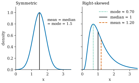
Two density curves. On the left, a symmetric bell curve where mean, median and mode all sit at the peak, 1.5. On the right, a curve with a long right tail: the mode is at about 0.70, the median at 1, and the mean further right at about 1.20. — Left: normal density with mean 1.5 and standard deviation 0.4; mean, median and mode coincide. Right: right-skewed log-normal density (the logarithm of the variable has mean 0 and standard deviation 0.6); mode ≈ 0.70 (dotted), median = 1 (solid), mean ≈ 1.20 (dashed).

In the right-skewed curve, the long tail of large values pulls the mean upwards while the median, which only counts how much area lies on each side, moves less. The mode sits at the peak. This is the typical pattern for incomes, house prices, and waiting times: mode < median < mean. For a left-skewed distribution the order is usually reversed.

This ordering is a useful heuristic, not a theorem. It holds for many common distributions but can fail, especially for discrete data or distributions with more than one peak. For example, the dataset

1,\; 1,\; 1,\; 3,\; 3,\; 3,\; 8

has a long right tail (one value far above the rest), yet its mean $20/7 \approx 2.86$ is below its median of 3. Among standard distributions, a Poisson distribution with mean 1.7 is right-skewed but has median 2. So use the gap between mean and median as a hint about skew, and confirm by looking at a histogram.

Which one to use

Roughly symmetric numerical data without extreme values: the mean, usually reported with the standard deviation. It uses all the information and has convenient mathematical properties.
Skewed data or data with outliers: the median, usually with the interquartile range. Median household income is reported for this reason.
Totals matter: the mean, since total = mean × number of observations.
Categorical data, or the most common value is what matters: the mode (the most common shoe size is what a shop should stock most of).

When in doubt, report both the mean and the median. If they differ a lot, say so and show a plot.

Common misunderstandings

“The average is what a typical member experiences.” Only if the distribution is roughly symmetric. In the salary example, six of seven employees earn below the mean.

“Mean > median proves the data are right-skewed.” It is a hint, not a proof; the example above shows the rule can fail.

“The median ignores the data.” It uses every observation to decide what is in the middle; it just ignores how far the outer values are from the centre.

“The mean of a sample is the population mean.” The sample mean $\bar{x}$ is an estimate of the population mean $\mu$ and changes from sample to sample. How much it changes is described by its sampling distribution.