Hypothesis Testing

A procedure for deciding whether data are inconsistent enough with a default claim about a population to reject that claim.

Prerequisites: Sampling Distributions, Normal Distribution, Central Limit Theorem.

A hypothesis test is a procedure for deciding whether sample data provide enough evidence against a default claim about a population, called the null hypothesis. If data like ours would be very unusual were the null hypothesis true, we reject it; otherwise we do not.

Hypothesis tests are used to check whether a production process is on target, whether a new treatment differs from a placebo, or whether two groups differ. They give a disciplined answer to the question “could this pattern plausibly be just random variation?”, with a known rate of false alarms.

Intuition

A machine is supposed to fill packages with 500 g of flour. You weigh 25 packages and find an average of 498.2 g. Is the machine underfilling, or is 1.8 g below target just the kind of difference that random variation produces anyway?

A hypothesis test answers by temporarily assuming that nothing is wrong (the true mean fill is exactly 500 g) and asking how surprising the observed average would be under that assumption. If it would be very surprising, the assumption looks doubtful and we reject it. If it would not be surprising, the data are consistent with the machine being on target, though they do not prove it.

The logic resembles a criminal trial. The defendant is presumed innocent (the null hypothesis), and the verdict is “guilty” only if the evidence is strong enough. A verdict of “not guilty” does not mean the defendant was shown to be innocent.

The ingredients of a test

Hypotheses. The null hypothesis $H_0$ is the default claim, usually “no effect” or “no difference”, stated in terms of a population parameter. The alternative hypothesis $H_1$ (also written $H_a$ ) is what we conclude if we reject $H_0$ . For the flour machine, with $\mu$ the true mean fill weight,

H_0: \mu = 500 \qquad \text{versus} \qquad H_1: \mu \ne 500.

Hypotheses are statements about the population, never about the sample: there is no doubt that the sample mean is 498.2 g.

Test statistic. A number $T$ computed from the data that measures how far the data depart from $H_0$ . We write $t_{\text{obs}}$ for its observed value. For a mean with known population standard deviation $\sigma$ , the usual choice is the z statistic

Z = \frac{\bar{X} - \mu_0}{\sigma / \sqrt{n}},

where $\mu_0$ is the value of $\mu$ under $H_0$ (here 500), $\bar{X}$ is the sample mean, and $\sigma/\sqrt{n}$ is its standard error. It counts how many standard errors the sample mean lies from $\mu_0$ .

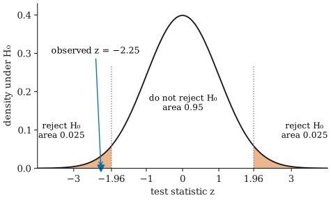
Null distribution. The sampling distribution of the test statistic, computed on the assumption that $H_0$ is true. If the data are normal, or $n$ is large enough for the central limit theorem, then under $H_0$ the z statistic has a standard normal distribution.

Significance level. A threshold $\alpha$ , chosen before looking at the data, for how often we are willing to reject $H_0$ when it is in fact true. The conventional choice is $\alpha = 0.05$ , but there is nothing special about it.

Rejection region. The set of values of the test statistic that lead to rejecting $H_0$ . It is chosen so that, under $H_0$ , the test statistic falls in it with probability $\alpha$ . For a two-sided z test at $\alpha = 0.05$ , the rejection region is $|z| > 1.96$ , because $P(|Z| > 1.96) \approx 0.05$ for a standard normal $Z$ .

Decision. If $t_{\text{obs}}$ falls in the rejection region, reject $H_0$ . Otherwise, do not reject $H_0$ .

A standard normal curve centred at zero. The two tails beyond minus 1.96 and plus 1.96 are shaded and labelled as rejection regions, each with area 0.025. The observed statistic, minus 2.25, is marked inside the left rejection region. — Two-sided z test at α = 0.05. Under H₀ the test statistic is standard normal; the shaded tails beyond ±1.96 together have probability 0.05. The observed z = −2.25 from the flour example falls in the left rejection region, so H₀ is rejected.

An equivalent way to make the decision is through the p-value: the probability, computed assuming $H_0$ is true, of a test statistic at least as extreme as the one observed. Reject $H_0$ exactly when the p-value is at most $\alpha$ . The p-value adds information the yes-or-no decision hides, namely how far into the tail the observation fell.

Worked example

Return to the flour machine. From long experience, individual fill weights vary with standard deviation $\sigma = 4$ g. A sample of $n = 25$ packages has mean $\bar{x} = 498.2$ g. Test $H_0: \mu = 500$ against $H_1: \mu \ne 500$ at $\alpha = 0.05$ .

Step 1: standard error.

\frac{\sigma}{\sqrt{n}} = \frac{4}{\sqrt{25}} = 0.8 \text{ g}.

Step 2: test statistic.

z = \frac{498.2 - 500}{0.8} = \frac{-1.8}{0.8} = -2.25.

The sample mean is 2.25 standard errors below the target.

Step 3: compare with the rejection region. Since $|{-2.25}| = 2.25 > 1.96$ , the statistic falls in the rejection region.

Step 4: decide and state the conclusion in context. Reject $H_0$ at the 5% level. The data give evidence that the machine’s mean fill differs from 500 g; the estimate suggests it is underfilling by roughly 1.8 g. The two-sided p-value is $2\,\Phi(-2.25) \approx 0.024$ , where $\Phi$ is the standard normal CDF.

If σ were unknown. We would replace $\sigma$ by the sample standard deviation $s$ and compare the statistic $(\bar{x} - \mu_0)/(s/\sqrt{n})$ with the $t$ distribution with $n - 1 = 24$ degrees of freedom, whose two-sided 5% critical value is about $2.064$ instead of $1.96$ . This is the one-sample t test; it is the version used most often in practice.

Type I and type II errors

A test can be wrong in two ways.

	$H_0$ true	$H_0$ false
Reject $H_0$	Type I error (false alarm), probability $\alpha$	Correct decision, probability $1 - \beta$ (the power)
Do not reject $H_0$	Correct decision, probability $1 - \alpha$	Type II error (missed effect), probability $\beta$

A type I error is rejecting a true null hypothesis. Its probability is the significance level $\alpha$ , which we control directly.
A type II error is failing to reject a false null hypothesis. Its probability is written $\beta$ .
The power of a test, $1 - \beta$ , is the probability of correctly rejecting $H_0$ when it is false.

Power is not a single number: it depends on how far the truth is from $H_0$ . For the flour test above ( $\sigma = 4$ , $n = 25$ , $\alpha = 0.05$ ), the power is about 0.24 if the true mean is 499 g and about 0.71 if it is 498 g. Small departures are hard to detect. Power increases with the size of the true effect, with the sample size $n$ , and with $\alpha$ , and decreases with the population standard deviation $\sigma$ . Lowering $\alpha$ to reduce false alarms, with $n$ fixed, raises $\beta$ : there is a trade-off between the two kinds of error. Studies are often planned by choosing $n$ large enough to give, say, 80% power for the smallest effect that would matter.

One-sided and two-sided tests

The alternative $H_1: \mu \ne 500$ is two-sided: departures in either direction count as evidence against $H_0$ , and the rejection region is split between both tails.

If only one direction matters, for example if the regulator only cares about underfilling, a one-sided alternative $H_1: \mu < 500$ can be used. All of $\alpha$ is then placed in one tail: at $\alpha = 0.05$ the rejection region is $z < -1.645$ . A one-sided test has more power in the chosen direction but cannot detect a departure in the other direction.

The choice between one- and two-sided tests must be made before seeing the data, based on the question being asked. Choosing the direction after seeing which way the data point effectively doubles the type I error rate.

Tests and confidence intervals

Two-sided tests and confidence intervals are two views of the same calculation. For the z test above, a two-sided test at level $\alpha$ rejects $H_0: \mu = \mu_0$ exactly when $\mu_0$ lies outside the $100(1-\alpha)\%$ confidence interval $\bar{x} \pm z^* \sigma/\sqrt{n}$ .

In the flour example, the 95% interval is $498.2 \pm 1.96 \times 0.8$ , or about 496.6 g to 499.8 g. It does not contain 500, matching the decision to reject. The interval also shows what the test alone does not: which values of $\mu$ are consistent with the data.

This exact correspondence holds when the test and the interval are built from the same statistic and the same standard error, as here. For some other procedures (for example the Wald interval for a proportion paired with a test that uses the null value in its standard error) the two can occasionally disagree near the boundary. A one-sided test corresponds to a one-sided confidence bound rather than to the usual two-sided interval.

Common misunderstandings

“Failing to reject H₀ means H₀ is true.” It means only that the data were not inconsistent enough with $H_0$ to reject it. A small sample may simply lack the power to detect a real effect. “Not guilty” is not “innocent”. The p-values article discusses this further under misinterpretations.

“Rejecting H₀ proves H₁.” A test controls the long-run rate of false rejections; it does not prove anything. About 5% of tests of true null hypotheses at $\alpha = 0.05$ will reject.

“α is the probability that H₀ is true after we reject it.” $\alpha$ is the probability of rejecting given that $H_0$ is true. The probability that $H_0$ is true given a rejection is a different conditional probability and cannot be computed from $\alpha$ alone.

“Statistically significant means important.” With a large enough sample, even a trivial difference, such as a fill weight 0.05 g below target, produces a significant result. Always report the estimated size of the effect, ideally with a confidence interval.

“The hypotheses can be adjusted after looking at the data.” Choosing the alternative, the significance level, or which test to run after seeing the data invalidates the stated error rates.