Law of Large Numbers

As a sample grows, its average gets closer and closer to the expected value.

Prerequisites: Expected Value, Variance of a Random Variable, Statistical Independence.

The law of large numbers says that the average of many independent repetitions of the same random experiment gets close to the expected value, and gets closer as the number of repetitions grows. Toss a fair coin ten times and you may well see 7 heads; toss it ten thousand times and the proportion of heads will almost certainly be very near one half.

It is the reason averages are useful at all. It justifies estimating a population mean by a sample mean, interpreting probabilities as long-run frequencies, and running simulations to approximate quantities that are hard to compute exactly.

Intuition

Each individual outcome is unpredictable, but in an average, high and low values partly cancel. With few observations, one or two unusual values can pull the average far from the centre. With many observations, any single value has a weight of only $1/n$, so it can move the average very little, and the overall result is dominated by the typical behaviour of the process.

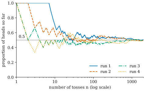
The figure shows four simulated sequences of coin tosses. After a handful of tosses the proportion of heads is all over the place: one run starts with seven heads in a row. As the tosses accumulate, the lines settle into an ever narrower band around 0.5. No single run is forced to reach 0.5 exactly; they simply wander less and less.

Statement

Let $X_1, X_2, \dots$ be independent and identically distributed (iid) random variables, each with finite mean $\mu = \E[X_i]$. Write the average of the first $n$ of them as

$$\bar{X}_n = \frac{1}{n} \sum_{i=1}^n X_i.$$

The subscript $n$ is a reminder that the average depends on how many observations it uses. For coin tosses, $X_i = 1$ for heads and $0$ for tails, so $\mu = 0.5$ and $\bar{X}_n$ is the proportion of heads.

Weak law of large numbers. For every tolerance $\varepsilon > 0$, however small,

$$P\big(|\bar{X}_n - \mu| > \varepsilon\big) \to 0 \quad \text{as } n \to \infty.$$

In words: pick any margin of error you like. The probability that the average misses $\mu$ by more than that margin becomes as small as you want once $n$ is large enough. This kind of convergence is called convergence in probability.

There is also a strong law of large numbers, which says that, with probability 1, the sequence of averages $\bar{X}_1, \bar{X}_2, \dots$ actually converges to $\mu$. Under the same assumptions, both laws hold. The distinction matters in advanced probability; for most purposes, “the average converges to the mean” is the message of both.

The assumptions

• Identical distribution with a finite mean. If the mean does not exist, there is nothing to converge to. The standard example is the Cauchy distribution, whose tails are so heavy that it has no mean: the average of $n$ Cauchy variables has exactly the same distribution as a single one, and it never settles down.
• Independence, or at least not too much dependence. If every observation shares a common error (for example, a miscalibrated instrument), averaging more readings converges to the wrong value. Independence is what lets the errors cancel.

Why it is true

When the variance $\sigma^2$ is also finite, there is a short proof. From the article on sampling distributions, $\E[\bar{X}_n] = \mu$ and $\Var(\bar{X}_n) = \sigma^2/n$. Chebyshev’s inequality says that any random variable is unlikely to be many standard deviations from its mean: for any $\varepsilon > 0$,

$$P\big(|\bar{X}_n - \mu| \ge \varepsilon\big) \le \frac{\Var(\bar{X}_n)}{\varepsilon^2} = \frac{\sigma^2}{n\varepsilon^2}.$$

The right-hand side goes to $0$ as $n$ grows, which proves the weak law. The proof also shows why it works: the variance of the average shrinks like $1/n$. (The law still holds without a finite variance, but the proof is harder.)

Worked example

For a fair coin, $\mu = 0.5$ and $\sigma^2 = 0.5 \times 0.5 = 0.25$. How likely is the proportion of heads to be within 0.05 of one half?

The exact probabilities, computed from the binomial distribution, are:

With 10 tosses, the only proportion in the band is exactly 5 heads, which happens about a quarter of the time. With 1,000 tosses, missing the band is roughly a 1-in-700 event.

Chebyshev’s inequality gives a guaranteed, but much cruder, bound. For $n = 1000$ and $\varepsilon = 0.05$:

$$P\big(|\bar{X}_n - 0.5| \ge 0.05\big) \le \frac{0.25}{1000 \times 0.05^2} = 0.1.$$

The true probability is about 0.0017. Chebyshev is useful for proving that convergence happens, not for computing how fast; the central limit theorem gives far better approximations.

Common misunderstandings

“After a run of heads, tails is due.” This is the gambler’s fallacy. Coin tosses are independent: the coin has no memory, and the probability of heads on the next toss is still 0.5. The law of large numbers does not work by correcting past deviations. It works by diluting them. Suppose the first 10 tosses give 8 heads, 3 more than expected. Over the next 990 tosses we expect 495 heads, so after 1,000 tosses we expect $(8 + 495)/1000 = 0.503$. The 3 extra heads are still there; they just matter less and less in the average.

“The number of heads will get close to half the number of tosses.” The proportion converges; the count need not. The difference between the number of heads and $n/2$ typically grows like $\sqrt{n}$ (its standard deviation is $0.5\sqrt{n}$). In the figure, after 2,000 tosses the four runs are off by +10, −11, −8 and −15 heads, yet their proportions are all within 0.008 of 0.5.

“The law of large numbers says the average is approximately normal.” That is the central limit theorem, a different and more detailed result. The law of large numbers says where the average goes (to $\mu$). The central limit theorem describes the shape and size of its fluctuations around $\mu$ along the way.

“With enough data, any average is accurate.” Only if the data are independent draws from the process you care about. A huge biased sample converges, reliably, to the wrong answer.

Further reading

• Joseph K. Blitzstein and Jessica Hwang, Introduction to Probability, 2nd ed., CRC Press, 2019. Covers both laws of large numbers and Chebyshev’s inequality, with simulations.
• David Freedman, Robert Pisani, and Roger Purves, Statistics, 4th ed., W. W. Norton, 2007. A nonmathematical discussion of chance error and why the count of heads drifts while the proportion settles.

Related articles

• Sampling Distributions — The distribution of a statistic, such as the sample mean, over all the samples that could have been drawn.
• Central Limit Theorem — The mean of many independent observations is approximately normally distributed, whatever the shape of the population.
• Point Estimation — Using a single number computed from a sample to estimate an unknown population parameter, and judging how good that rule is.