P-values and Statistical Significance

The probability, assuming the null hypothesis and the model are true, of a result at least as extreme as the one observed.

Prerequisites: Hypothesis Testing, Bernoulli and Binomial Distributions.

A p-value is the probability, calculated assuming that the null hypothesis and the rest of the statistical model are true, of getting a test statistic at least as extreme as the one actually observed. A small p-value says the data would be unusual if the null hypothesis were true; a large one says they would not.

P-values are among the most reported numbers in science, and among the most misread. This article defines them, works through an example, and then covers what a p-value does not tell you, following the American Statistical Association’s 2016 statement on p-values.

Intuition

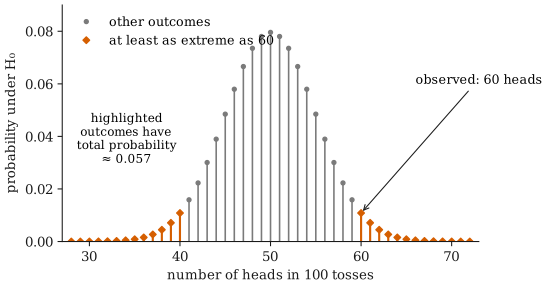
You suspect a coin is biased, so you toss it 100 times and get 60 heads. A fair coin would give about 50 on average, but never exactly 50 every time. Is 60 far enough from 50 to make you doubt the coin is fair?

The p-value answers a precise version of that question: if the coin were fair, how often would 100 tosses give a result at least as lopsided as this one? Here “at least as lopsided” means 60 or more heads, or, by symmetry, 40 or fewer. If such results were common under fairness, 60 heads is not surprising. If they were rare, either something rare happened, or the coin is not fair (or some other part of the model, such as independence of tosses, is wrong).

Definition

Consider a hypothesis test with null hypothesis $H_0$ and test statistic $T$ , where values of $T$ further from what $H_0$ predicts count as more extreme. Let $t_{\text{obs}}$ be the value of $T$ calculated from the observed data. The p-value is

p = P(T \text{ at least as extreme as } t_{\text{obs}}),

where the probability is computed using the distribution of $T$ under $H_0$ , the null distribution.

What “at least as extreme” means depends on the alternative hypothesis $H_1$ :

Two-sided alternatives count departures in both directions. For a statistic whose null distribution is symmetric about the value $H_0$ predicts, the two-sided p-value is twice the one-tail probability beyond the observed value.
One-sided alternatives count only departures in the direction stated by $H_1$ .

Three things to notice about the definition:

The p-value is computed assuming $H_0$ is true. It is a probability about data, not about hypotheses.
It depends on the whole model, not just $H_0$ : for the coin, that the tosses are independent and have the same probability of heads. A small p-value can signal a problem with any of these assumptions.
It involves results at least as extreme as the one observed, not just the observed result itself. Any single exact outcome may be unlikely; what matters is how far into the tail it lies.

Worked example

Toss a coin $n = 100$ times and observe 60 heads. Let $X$ be the number of heads. Test

H_0: \theta = 0.5 \qquad \text{versus} \qquad H_1: \theta \ne 0.5,

where $\theta$ is the probability of heads on a single toss. (We write $\theta$ rather than the usual $p$ to avoid a clash with the p-value.)

Step 1: the null distribution. If $H_0$ is true and the tosses are independent, $X$ has a binomial distribution with $n = 100$ trials and success probability $0.5$ . It is centred at $50$ and symmetric about $50$ .

Step 2: which outcomes are at least as extreme? The observed count is $10$ away from $50$ . Outcomes at least as far from $50$ are $X \ge 60$ and $X \le 40$ .

Step 3: add up their probabilities (exact calculation). Using the binomial PMF,

P(X \ge 60) = \sum_{k=60}^{100} \binom{100}{k} 0.5^{100} \approx 0.0284.

By symmetry $P(X \le 40)$ is the same, so the exact two-sided p-value is

p = P(X \le 40) + P(X \ge 60) \approx 2 \times 0.0284 \approx 0.057.

If the coin were fair, about 5.7% of experiments of 100 tosses would be at least this lopsided.

Stems showing the binomial probabilities for 28 to 72 heads in 100 fair tosses, peaking at 50. The stems at 40 or fewer and at 60 or more are highlighted in a different colour and marker; together they make up about 0.057 of the probability. — Null distribution of the number of heads in 100 tosses of a fair coin, Binomial(100, 0.5), shown for 28 to 72 heads. The highlighted outcomes (40 or fewer heads, or 60 or more) are at least as extreme as the observed 60; their total probability, the exact two-sided p-value, is about 0.057.

A normal approximation. Many textbooks instead approximate the binomial by a normal distribution with the same mean, $100 \times 0.5 = 50$ , and the same standard deviation, $\sqrt{100 \times 0.5 \times 0.5} = 5$ . The z statistic is $z = (60 - 50)/5 = 2$ , and the two-sided p-value is $2\,(1 - \Phi(2)) \approx 0.046$ , where $\Phi$ is the standard normal CDF. With a continuity correction (using $59.5$ in place of $60$ , since the count is discrete), $z = 1.9$ and the p-value is about $0.057$ , close to the exact answer.

Notice what just happened. The exact p-value is just above $0.05$ and the uncorrected approximation is just below it. The evidence is the same in both cases; only the arithmetic differs. This is a good reason not to treat $0.05$ as a cliff.

Statistical significance

Before collecting data, the analyst may choose a significance level $\alpha$ , conventionally $0.05$ . If $p \le \alpha$ , the result is called statistically significant at level $\alpha$ , and $H_0$ is rejected. This rule is identical to checking whether the test statistic falls in the rejection region of the corresponding test.

The rule has a useful guarantee. If $H_0$ and the model are true, the probability of getting $p \le \alpha$ is at most $\alpha$ . So declaring significance whenever $p \le 0.05$ produces false alarms in at most about 5% of tests of true null hypotheses. (For a discrete statistic such as a binomial count, the rate is typically a little below $\alpha$ .)

“Statistically significant” is a technical term. It means only that the data are hard to reconcile with $H_0$ under the model. It does not mean important, large, or proven.

Common misunderstandings

In 2016 the American Statistical Association published a statement on p-values (Wasserstein and Lazar, listed below) to address widespread misuse. Its six principles say, in brief: p-values can indicate how incompatible data are with a specified model; they do not measure the probability that a hypothesis is true, or the probability that the data were produced by chance alone; conclusions should not rest only on whether a p-value passes a threshold; proper inference requires full reporting and transparency; a p-value does not measure the size or importance of an effect; and by itself a p-value is not a good measure of evidence about a model or hypothesis. The misunderstandings below follow from these principles.

“The p-value is the probability that H₀ is true.” It is not. The p-value is a probability about the data computed assuming $H_0$ is true, roughly $P(\text{data this extreme} \mid H_0)$ . The probability that $H_0$ is true given the data is the reverse conditional probability, and getting it requires Bayes’ theorem and a prior probability for $H_0$ . In the coin example, $p \approx 0.057$ does not mean there is a 5.7% chance the coin is fair.

“The p-value is the probability that the result is due to chance.” This is the same mistake in different words. The calculation already assumes that chance alone (under $H_0$ ) is at work; it cannot also give the probability of that assumption.

“A small p-value means a large or important effect.” Statistical significance is not practical significance. The p-value depends on the sample size as well as on the effect. Toss a coin a million times and get 50.2% heads: the z statistic is $(0.502 - 0.5)/(0.5/\sqrt{1\,000\,000}) = 4$ and the two-sided p-value is about $0.00006$ , yet a bias of 0.2 percentage points is irrelevant for most purposes. Always report the effect size, the estimated magnitude of the effect, preferably with a confidence interval.

“p > 0.05 shows there is no effect.” A large p-value means the data are reasonably consistent with $H_0$ , but they may be just as consistent with a substantial effect, especially in a small study with low power. Absence of evidence is not evidence of absence. A confidence interval shows which effect sizes remain plausible.

“p = 0.049 and p = 0.051 lead to opposite conclusions.” They represent nearly identical evidence. The worked example above produced p-values on either side of 0.05 from the same data, depending only on the method of calculation. Report the p-value itself rather than only “significant” or “not significant”.

“If I run many tests, a small p-value is still meaningful on its own.” Each test of a true null hypothesis at $\alpha = 0.05$ has a 5% chance of a false alarm, and those chances add up. With 20 independent tests of true null hypotheses, the probability that at least one gives $p \le 0.05$ is $1 - 0.95^{20} \approx 0.64$ . Trying many analyses, outcomes, subgroups, or stopping rules and reporting only the ones that “worked” is called p-hacking or data dredging, and it makes reported p-values meaningless. Remedies include deciding the analysis in advance, reporting every test performed, and adjusting for multiple comparisons (for example, the Bonferroni correction, which tests each of $m$ hypotheses at level $\alpha/m$ ).