Bernoulli and Binomial Distributions

The distributions of a single yes/no trial and of the number of successes in a fixed number of independent trials.

Prerequisites: Probability Distributions, Statistical Independence, Expected Value.

The Bernoulli distribution describes a single trial with two outcomes, “success” or “failure”, such as one coin toss or one free throw. The binomial distribution describes the number of successes in a fixed number of such trials when the trials are independent and each has the same chance of success.

Together they are the basic model for counting yes/no outcomes: how many patients respond to a treatment, how many of 20 emails are spam, how many of 10 free throws go in. Both are discrete distributions, so they assign probabilities to separate values through a probability mass function.

Intuition

Suppose a basketball player makes each free throw with probability $0.7$ and takes 10 shots. The number of baskets could be anything from 0 to 10, but not all values are equally likely. Around 7 is typical. Exactly 10 requires every shot to go in, which is rare. Exactly 7 can happen in many ways (any 7 of the 10 shots could be the successful ones), which is why values near the middle collect most of the probability.

The binomial distribution makes this counting precise. It has two ingredients: the probability of one particular sequence of successes and failures, and the number of sequences that give the same total.

The Bernoulli distribution

A random variable $X$ has a Bernoulli distribution with parameter $p$, written $X \sim \text{Bernoulli}(p)$, if it takes the value $1$ (success) with probability $p$ and the value $0$ (failure) with probability $1 - p$, where $0 \le p \le 1$:

$$P(X = 1) = p, \qquad P(X = 0) = 1 - p.$$

Coding success as $1$ and failure as $0$ is a convenient choice: the variable then counts successes in one trial, and averages of such variables are proportions.

Its expected value and variance follow directly from the definitions:

$$\E[X] = 1 \cdot p + 0 \cdot (1-p) = p,$$

and since $X^2 = X$ when $X$ is $0$ or $1$, $\E[X^2] = p$, so

$$\Var(X) = \E[X^2] - (\E[X])^2 = p - p^2 = p(1-p).$$

The variance is largest at $p = 0.5$, where the outcome is most uncertain, and zero at $p = 0$ or $p = 1$, where there is no uncertainty at all.

The binomial distribution

Let $X$ be the number of successes in $n$ trials, where

1. the number of trials $n$ is fixed in advance,
2. each trial has two outcomes, success or failure,
3. every trial has the same probability of success $p$, and
4. the trials are independent.

Then $X$ has a binomial distribution with parameters $n$ (a positive integer) and $p$ (with $0 \le p \le 1$), written $X \sim \text{Binomial}(n, p)$. Its probability mass function is

$$P(X = k) = \binom{n}{k} p^k (1-p)^{n-k}, \qquad k = 0, 1, \dots, n.$$

Reading the formula

• $p^k (1-p)^{n-k}$ is the probability of one particular sequence with $k$ successes and $n - k$ failures, for example success, success, failure, … By independence, the probabilities of the individual trials multiply. Every sequence with $k$ successes has this same probability, whatever the order.
• $\binom{n}{k} = \dfrac{n!}{k!\,(n-k)!}$, read “$n$ choose $k$”, is the number of different sequences with exactly $k$ successes, that is, the number of ways to choose which $k$ of the $n$ trials are the successes. Here $n! = n \times (n-1) \times \dots \times 1$, and $0! = 1$.

Multiplying gives the total probability of all the sequences with $k$ successes. The Bernoulli distribution is the special case $n = 1$.

Mean and variance

The cleanest way to find the mean and variance is to write $X$ as a sum. Let $X_i = 1$ if trial $i$ is a success and $0$ otherwise. Each $X_i \sim \text{Bernoulli}(p)$, and

$$X = X_1 + X_2 + \dots + X_n.$$

Expectation is linear, so the expected value of a sum is the sum of the expected values:

$$\E[X] = \E[X_1] + \dots + \E[X_n] = np.$$

Because the trials are independent, the variance of the sum is also the sum of the variances:

$$\Var(X) = \Var(X_1) + \dots + \Var(X_n) = np(1-p).$$

The standard deviation is $\sqrt{np(1-p)}$. As a sanity check, with $p = 0$ or $p = 1$ the count is certain ($0$ or $n$) and the variance formula correctly gives $0$.

How the shape depends on n and p

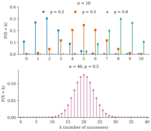
• The distribution is centred near $np$: around $2$, $5$, and $8$ in the top panel.
• With $p = 0.5$ it is symmetric. With $p < 0.5$ it is skewed to the right (a longer tail toward large counts), and with $p > 0.5$ it is skewed to the left. The distributions for $p$ and $1 - p$ are mirror images, because counting successes with probability $p$ is the same as counting failures with probability $1 - p$.
• As $n$ grows, the distribution becomes wider in absolute terms (the standard deviation grows like $\sqrt{n}$) and more bell-shaped, as in the bottom panel.

Worked example

A player makes each free throw with probability $p = 0.7$, independently of the other shots, and takes $n = 10$ shots. Let $X$ be the number made, so $X \sim \text{Binomial}(10, 0.7)$.

Step 1: mean and spread. $\E[X] = 10 \times 0.7 = 7$ and $\Var(X) = 10 \times 0.7 \times 0.3 = 2.1$, so the standard deviation is $\sqrt{2.1} \approx 1.45$ baskets.

Step 2: exactly 8 baskets. The number of ways to choose which 8 of the 10 shots go in is $\binom{10}{8} = 45$. Each such sequence has probability $0.7^8 \times 0.3^2$. So

$$P(X = 8) = 45 \times 0.7^8 \times 0.3^2 \approx 45 \times 0.05765 \times 0.09 \approx 0.2335.$$

Step 3: at least 8 baskets. Add the probabilities of 8, 9, and 10:

$$P(X = 9) = 10 \times 0.7^9 \times 0.3 \approx 0.1211, \qquad P(X = 10) = 0.7^{10} \approx 0.0282.$$

$$P(X \ge 8) \approx 0.2335 + 0.1211 + 0.0282 = 0.3828.$$

So the player makes 8 or more about 38% of the time. Although 7 is the single most likely value, its probability is only about $0.27$: no single count is very likely.

When the assumptions fail

The binomial model needs all four conditions above. Common ways they break:

• Probability not constant. A player who tires makes later shots less often, so the count is no longer binomial. A particularly common case is a $p$ that changes between occasions: a player has good days and bad days, and all 10 shots on one day share that day’s form. Counts collected over many days are then more spread out than a single binomial predicts.
• Trials not independent. Hot and cold streaks, or students in the same class who influence each other’s answers, also tend to inflate the spread.
• Sampling without replacement. Drawing 10 cards from a deck and counting hearts is not binomial, because each draw changes the deck. When the sample is a small fraction of a large population, the binomial is still a good approximation.
• Number of trials not fixed. If you keep tossing until the third head, the number of tosses is random and the binomial model does not apply.

Approximations

Normal approximation. When $n$ is large and $p$ is not too close to $0$ or $1$, the binomial distribution is close to a normal distribution with the same mean $np$ and variance $np(1-p)$. This is a consequence of the central limit theorem, since $X$ is a sum of $n$ independent Bernoulli variables. A common rule of thumb is to require $np \ge 10$ and $n(1-p) \ge 10$. Because the binomial is discrete, the approximation is better with a continuity correction: treat the integer $k$ as the interval from $k - 0.5$ to $k + 0.5$. For 100 tosses of a fair coin, $P(X \le 45)$ is about $0.1841$ exactly, and the normal approximation $\Phi\big((45.5 - 50)/5\big)$ gives about $0.1841$ as well.

Poisson approximation. When $n$ is large and $p$ is small, so that successes are rare, the binomial is close to a Poisson distribution with mean $\lambda = np$.

Common misunderstandings

“The most likely count happens most of the time.” In the example, 7 is the most likely number of baskets, but it happens only about 27% of the time. With larger $n$ the probability of any single exact count gets smaller still.

“Any count of successes is binomial.” Only if the number of trials is fixed, the trials are independent, and the success probability is the same for each. Check these before using the formulas, particularly the standard deviation, which is too small when the assumptions fail.

“Bernoulli and binomial are unrelated distributions.” A Bernoulli variable is a binomial variable with $n = 1$, and every binomial variable is a sum of independent Bernoulli variables.

“The variance is np.” That is the Poisson variance. The binomial variance $np(1-p)$ is always smaller than $np$ when $0 < p$; the two are close only when $p$ is small.

Further reading

• Joseph K. Blitzstein and Jessica Hwang, Introduction to Probability, 2nd ed., CRC Press, 2019. Derives the binomial distribution through counting and through sums of indicator variables.
• David M. Diez, Mine Çetinkaya-Rundel, and Christopher D. Barr, OpenIntro Statistics, 4th ed., 2019. Free online; includes worked binomial examples and the normal approximation.

Related articles

• Poisson Distribution — The distribution of the number of events in a fixed interval when events occur independently at a constant average rate.
• Normal Distribution — The bell-shaped continuous distribution described by a mean and a standard deviation.
• Variance of a Random Variable — The expected squared distance of a random variable from its mean, measuring how spread out its distribution is.
• Central Limit Theorem — The mean of many independent observations is approximately normally distributed, whatever the shape of the population.