Probability Distributions

A description of which values a random variable can take and how probability is spread over them.

Prerequisites: Introduction to Probability, Random Variables.

A probability distribution describes which values a random variable can take and how likely each value, or each range of values, is. It is the complete probabilistic description of an uncertain quantity: once you know the distribution, you can answer any question of the form “what is the probability that the value lands here?”

Distributions are the basic vocabulary of statistics. Statistical models are built by choosing a distribution for the data, and most of inference is about learning the unknown numbers, the parameters, that pin that distribution down.

Intuition

Think of probability as a fixed amount of sand, exactly one unit, that has to be spread over the possible values of a random variable. The distribution says where the sand goes.

If the variable can only take separate values, such as the number of heads in four coin tosses (0, 1, 2, 3, or 4), the sand is piled up in lumps at those values. Each lump is a probability.
If the variable can take any value in a range, such as a person’s height, the sand is spread out smoothly, like a layer of varying thickness. No single point holds any sand by itself; only stretches of the line do. The thickness at a point is the density.

These two situations are handled with two different tools, the probability mass function and the probability density function. A third tool, the cumulative distribution function, works for both.

Left column: the number of heads in four fair coin tosses has probabilities 1/16, 4/16, 6/16, 4/16 and 1/16, drawn as separate stems, and its CDF is a staircase that jumps by those amounts. Right column: the standard normal density is a smooth bell curve whose area between −1 and 1 is about 0.68, and its CDF rises smoothly from 0 to 1. — A discrete distribution (left: number of heads in 4 fair coin tosses) and a continuous one (right: the standard normal distribution). Top: the PMF gives probabilities as heights; the PDF gives probabilities as areas. Bottom: both CDFs rise from 0 to 1, by jumps for the discrete variable and smoothly for the continuous one. Filled dots mark the value the step CDF takes at each jump.

Discrete distributions and the PMF

A random variable is discrete if it can take only a finite or countable list of separate values, such as $0, 1, 2, \dots$ Counts are the typical example.

A discrete distribution is described by its probability mass function (PMF)

p(x) = P(X = x),

the probability that the random variable $X$ takes exactly the value $x$ . A PMF must satisfy two conditions:

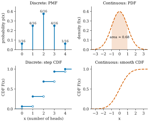
p(x) \ge 0 \quad \text{for every } x, \qquad \sum_{x} p(x) = 1,

where the sum runs over all possible values. The probability of a set of values is the sum of their masses. For the number of heads $X$ in four fair coin tosses (top-left panel above),

P(X \le 2) = p(0) + p(1) + p(2) = \frac{1}{16} + \frac{4}{16} + \frac{6}{16} = \frac{11}{16} \approx 0.69.

Continuous distributions and the PDF

A random variable is continuous if it can take any value in an interval, and the probability of every single exact value is $0$ . Heights, times, and temperatures are usually modelled this way.

A continuous distribution is described by a probability density function (PDF) $f(x)$ . Probabilities are areas under the density:

P(a \le X \le b) = \int_a^b f(x)\, dx.

A density must satisfy

f(x) \ge 0 \quad \text{for every } x, \qquad \int_{-\infty}^{\infty} f(x)\, dx = 1.

In the top-right panel above, the shaded area between $-1$ and $1$ is about $0.68$ , so a standard normal variable lands in that interval with probability about $0.68$ .

Density is not probability

The value $f(x)$ is not the probability that $X = x$ ; that probability is $0$ for every $x$ . A density is probability per unit length. For a small interval of width $h$ around $x$ ,

P(x \le X \le x + h) \approx f(x)\, h.

So a larger density means values near $x$ are more likely, but $f(x)$ itself has units of “probability per unit of $x$ ”. In particular, a density can be larger than $1$ . A variable spread evenly over the interval from $0$ to $0.5$ has density $2$ on that interval, because the area, $2 \times 0.5$ , must equal $1$ .

A practical consequence: for a continuous variable, $P(X \le b)$ and $P(X < b)$ are the same number, because the single point $b$ contributes nothing. For a discrete variable they can differ by $p(b)$ .

The cumulative distribution function

The cumulative distribution function (CDF) is defined the same way for every random variable:

F(x) = P(X \le x).

It answers “what is the probability of a value at most $x$ ?” Every CDF starts near $0$ on the far left, never decreases, and approaches $1$ on the far right.

For a discrete variable the CDF is a staircase: it is flat between possible values and jumps up by $p(x)$ at each possible value $x$ (bottom-left panel).
For a continuous variable the CDF is smooth, and its slope is the density: $F'(x) = f(x)$ wherever the derivative exists (bottom-right panel).

The CDF turns interval questions into a subtraction: $P(a < X \le b) = F(b) - F(a)$ , whatever the type of variable. It also gives quantiles: the median is the value where $F$ first reaches $0.5$ .

Parameters and families

Most named distributions are really families of distributions indexed by a few numbers called parameters. Choosing the parameter values picks out one member of the family.

For example, the normal distribution $\mathcal{N}(\mu, \sigma^2)$ has two parameters: the mean $\mu$ sets the location and the standard deviation $\sigma$ sets the spread. Every choice of $\mu$ and $\sigma > 0$ gives a different bell curve, but all of them share the same shape.

Parameters usually have constraints. A probability parameter must lie between $0$ and $1$ ; a rate or a standard deviation must be positive. Writing $X \sim \text{Family}(\text{parameters})$ reads “ $X$ has this distribution”. In statistics the parameters are typically unknown, and estimating them from data is the job of point estimation.

Two summaries of a distribution appear in almost every article: the expected value $\E[X]$ , its long-run average, and the variance $\Var(X)$ , its spread around that average.

Distributions in this section

Distribution	Type	Parameters	Possible values	Mean	Variance
Bernoulli	discrete	$0 \le p \le 1$	$0, 1$	$p$	$p(1-p)$
Binomial	discrete	$n \ge 1$ , $0 \le p \le 1$	$0, 1, \dots, n$	$np$	$np(1-p)$
Poisson	discrete	$\lambda > 0$	$0, 1, 2, \dots$	$\lambda$	$\lambda$
Uniform	continuous	$a < b$	$a \le x \le b$	$(a+b)/2$	$(b-a)^2/12$
Exponential	continuous	$\lambda > 0$	$x \ge 0$	$1/\lambda$	$1/\lambda^2$
Normal	continuous	$\mu$ , $\sigma > 0$	all real $x$	$\mu$	$\sigma^2$

Roughly: the Bernoulli and binomial distributions count successes in yes/no trials; the Poisson distribution counts events in a fixed interval; the uniform distribution spreads probability evenly over an interval; the exponential distribution describes waiting times; and the normal distribution describes measurements that cluster symmetrically around a typical value, as well as sums and averages of many independent pieces.

Common misunderstandings

“The height of a density curve is a probability.” It is a density. Only areas under the curve are probabilities, and a density can exceed $1$ ; see above.

“A continuous variable never takes any particular value, so nothing can happen.” Every observation is some particular value; the point is that no single value carries positive probability in advance. Intervals do, and they add up to $1$ .

“Drawing a smooth curve through a PMF gives its density.” A discrete variable has no density. Joining the stems of a PMF with a line suggests probability between the integers, where there is none.

“The data follow the distribution exactly.” A named distribution is a model. It is useful when its assumptions are close enough to the truth for the question at hand; checking that is part of the analysis.