Exponential Distribution

The distribution of the waiting time until the next event when events occur independently at a constant average rate.

Prerequisites: Probability Distributions, Poisson Distribution, Conditional Probability.

The exponential distribution describes the waiting time until the next event when events happen independently at a constant average rate: the time until the next call reaches a help desk, until the next customer walks in, or until a radioactive atom decays. It is a continuous distribution on the non-negative numbers, with short waits most likely and long waits progressively rarer.

It is the continuous partner of the Poisson distribution: the Poisson distribution counts events in an interval, and the exponential distribution measures the time between them. Its most distinctive property, memorylessness, says that if you have already waited a while, the remaining wait has the same distribution as if you had just started.

Intuition

Suppose customers arrive at a shop at an average rate of one every 4 minutes, independently of each other. At any moment, the chance that someone arrives in the next few seconds is the same, regardless of how long it has been since the last customer. Short gaps between customers are then common, because there is a steady chance of an arrival at every instant, starting right away. Long gaps happen too, but each extra minute of waiting requires one more minute with no arrival, so long gaps become rarer and rarer.

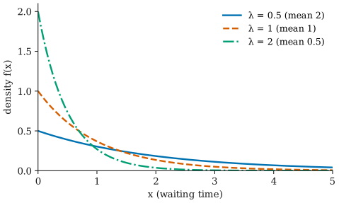
This gives the exponential shape: the density is highest at $0$ and decays by the same factor over each additional unit of time.

Three decreasing curves starting on the vertical axis. The curve with rate 2 starts highest, at 2, and falls fastest; the curve with rate 0.5 starts lowest, at 0.5, and decays slowly with a long tail. A higher rate means shorter typical waiting times. — Exponential densities for rates λ = 0.5, 1 and 2, with means 2, 1 and 0.5. Each density starts at height λ when x = 0 and decays toward zero; every curve encloses an area of 1.

Definition

A continuous random variable $X$ has an exponential distribution with rate $\lambda > 0$ , written $X \sim \text{Exponential}(\lambda)$ , if its probability density function is

f(x) = \lambda e^{-\lambda x}, \qquad x \ge 0,

and $f(x) = 0$ for $x < 0$ . Here:

$x$ is a possible waiting time, a non-negative real number;
$\lambda$ is the rate: the average number of events per unit time. If customers arrive at 15 per hour, $\lambda = 15$ per hour, or $0.25$ per minute.

Two conventions. Some books and software describe the same distribution by its mean (or scale) $\beta = 1/\lambda$ instead, writing the density as $f(x) = \frac{1}{\beta} e^{-x/\beta}$ . An exponential distribution “with parameter 4” might therefore have rate 4 or mean 4. For example, scipy.stats.expon uses scale $= 1/\lambda$ . Always check which one is meant.

The CDF and the survival function

Integrating the density gives the cumulative distribution function

F(x) = P(X \le x) = 1 - e^{-\lambda x}, \qquad x \ge 0.

Its complement, the probability of waiting longer than $x$ , is especially simple:

P(X > x) = e^{-\lambda x}.

This is called the survival function. Each extra unit of time multiplies the probability of still waiting by the same factor $e^{-\lambda}$ , which is what “exponential decay” means. The median is the time $m$ with $e^{-\lambda m} = 0.5$ , that is, $m = \log 2 / \lambda \approx 0.69 / \lambda$ . In radioactive decay, this median is the half-life.

Mean and variance

If $X \sim \text{Exponential}(\lambda)$ , then

\E[X] = \frac{1}{\lambda}, \qquad \Var(X) = \frac{1}{\lambda^2}.

The mean makes sense: if events occur at rate $\lambda$ per minute, the average gap between them is $1/\lambda$ minutes. Formally, integration by parts gives

\E[X] = \int_0^\infty x\, \lambda e^{-\lambda x}\, dx = \Big[ -x e^{-\lambda x} \Big]_0^\infty + \int_0^\infty e^{-\lambda x}\, dx = 0 + \frac{1}{\lambda}.

A second integration by parts gives $\E[X^2] = 2/\lambda^2$ , so $\Var(X) = 2/\lambda^2 - 1/\lambda^2 = 1/\lambda^2$ . The standard deviation equals the mean, $1/\lambda$ : waiting times are very variable relative to their average.

Because the distribution is skewed to the right, the median $0.69/\lambda$ is smaller than the mean $1/\lambda$ . About 63% of waits are shorter than the mean, since $P(X \le 1/\lambda) = 1 - e^{-1} \approx 0.632$ .

How the shape depends on the rate

There is only one shape; the rate stretches or squeezes it horizontally.

A larger rate $\lambda$ means events are more frequent, so waits are shorter: the density starts higher (at height $\lambda$ ) and falls faster.
A smaller rate means waits are longer: the density starts lower and has a longer tail.

As with any density, the starting height $\lambda$ can exceed $1$ ; only areas are probabilities.

Connection to the Poisson distribution

Consider events occurring independently at a constant average rate $\lambda$ per unit time, called a Poisson process. The number of events in any interval of length $t$ is $\text{Poisson}(\lambda t)$ .

Let $T$ be the waiting time until the first event. Waiting longer than $t$ means exactly that no event happens in the interval from $0$ to $t$ . The Poisson probability of zero events in that interval is $e^{-\lambda t}$ , so

P(T > t) = P(\text{no events in } [0, t]) = e^{-\lambda t}.

This is the exponential survival function with rate $\lambda$ . The same argument applies to the gap between any two consecutive events. So “counts are Poisson” and “gaps are exponential” are two descriptions of the same process.

Memorylessness

Suppose you have already waited $s$ minutes and nothing has happened. What is the chance you will wait more than $t$ further minutes? Using conditional probability, and the fact that waiting more than $s + t$ implies waiting more than $s$ ,

P(X > s + t \mid X > s) = \frac{P(X > s + t)}{P(X > s)} = \frac{e^{-\lambda (s + t)}}{e^{-\lambda s}} = e^{-\lambda t} = P(X > t).

The time already spent waiting is irrelevant: the remaining wait has the same exponential distribution as a fresh one. This is the memoryless property, and among continuous distributions only the exponential has it.

Intuitively, memorylessness is the constant-rate assumption seen from the other side. If the chance of an event in the next instant never depends on the past, then having waited a long time gives no reason to expect the event sooner. A radioactive atom does not “age”: an atom that has survived for a century is exactly as likely to decay in the next second as a newly formed one.

Worked example

Customers arrive at a shop independently, with an average gap of 4 minutes. The waiting time $X$ until the next customer, in minutes, is then exponential with rate $\lambda = 1/4 = 0.25$ per minute.

Step 1: mean and spread. $\E[X] = 4$ minutes and $\Var(X) = 1/0.25^2 = 16$ square minutes, so the standard deviation is also 4 minutes.

Step 2: a short wait. The probability that the next customer arrives within 2 minutes is

P(X \le 2) = 1 - e^{-0.25 \times 2} = 1 - e^{-0.5} \approx 0.393.

Step 3: a long wait. The probability of waiting more than 5 minutes is

P(X > 5) = e^{-0.25 \times 5} = e^{-1.25} \approx 0.287.

Step 4: memorylessness. Suppose 3 minutes have already passed with no customer. The probability of waiting more than 5 further minutes is

P(X > 8 \mid X > 3) = \frac{e^{-0.25 \times 8}}{e^{-0.25 \times 3}} = e^{-1.25} \approx 0.287,

the same as in Step 3. The 3 minutes already spent do not bring the next customer any closer.

Step 5: median. Half of all waits are shorter than $\log 2 / 0.25 \approx 2.77$ minutes, well below the 4-minute mean.

Where the exponential distribution appears

Times between random arrivals: calls, customers, requests to a web server, as long as the arrival rate is roughly constant over the period studied.
Radioactive decay: the lifetime of an individual unstable atom.
Reliability: the lifetime of components that fail through sudden random shocks rather than gradual wear, at a constant failure rate.
Queueing and simulation models: as the standard building block for random arrival and service times. A sample from it can be generated from a uniform random number $U$ as $-\log(1 - U)/\lambda$ .

Averages of many independent exponential waiting times are approximately normal, an example of the central limit theorem at work on a strongly skewed distribution.

Common misunderstandings

“Memorylessness applies to anything that fails.” It applies only when the failure rate is constant. Car tyres, human bodies, and machine bearings wear out: a 10-year-old pump is more likely to fail next month than a new one, so its lifetime is not exponential. Conversely, some products fail most often early on, through manufacturing defects. Assuming an exponential lifetime for ageing equipment underestimates the risk of failure late in life.

“I’ve waited a long time, so the bus must be due.” If buses run to a timetable, that is true, but then waiting times are not exponential. If arrivals really form a Poisson process, the waiting so far tells you nothing; this is the memoryless property.

“λ is the mean.” In this article, $\lambda$ is the rate and the mean is $1/\lambda$ . Many texts and programs use the mean as the parameter. Mixing the two conventions turns an average wait of 4 minutes into an average wait of a quarter of a minute.

“A typical wait is about as long as the average.” The density is highest at $0$ , and the median is only about 69% of the mean. Short waits are much more common than the mean suggests, balanced by occasional long ones.